If you’re a data engineer, you know handling semi-structured data from sources like IoT streams and application logs presents a costly dilemma. And, traditionally, you’ve been forced to choose between two suboptimal approaches: storing raw JSON as a STRING for maximum flexibility, or flattening it into a rigid STRUCT for performance.

The STRING approach offers you a schema-on-read philosophy but suffers from severe query latency, as every query must parse the entire JSON payload for every row. The STRUCT approach, on the other hand, delivers excellent query speed but sacrifices all flexibility, making any change to the source schema an expensive and tiring engineering task.  

However, the VARIANT data type then comes along to resolve this fundamental conflict between performance and flexibility. Initially pioneered by Snowflake in a proprietary form, the concept was later adopted and open-sourced by Databricks as “Open Variant” for Apache Spark and Delta Lake. This move created an open standard that delivered the schema-on-read flexibility of a STRING with the high query performance of a STRUCT, freeing the Lakehouse community from vendor lock-in.  

Under the Hood: What Makes the VARIANT Data Type Fast?

The remarkable performance of the VARIANT data type comes from a highly optimized binary encoding format in the underlying Parquet files. The open specification for VARIANT defines its physical representation in Parquet as a struct with two binary fields: metadata and value. They form a compressed, self-describing, query-optimized format.

The metadata field: a binary dictionary of all unique JSON keys in a given row. Each key (field name) is stored once per row and assigned a compact integer ID (called field ID).

The value field: stores the actual hierarchical JSON data in binary form, using the integer IDs from metadata instead of text keys. The structure is recursive, meaning objects or arrays can contain other nested VARIANT values (objects, arrays, or primitives), allowing arbitrarily deep nesting. For a path query (e.g., $.user.address.zip_code), the engine traverses the binary value field via stored offsets/pointers and consults the metadata dictionary only to map integer IDs to human-readable keys (e.g., "user", "address"). This ‘path navigation’ retrieves nested fields without parsing the entire JSON payload, bypassing the expensive full JSON parse step. And this is the primary bottleneck when querying JSON stored as a plain string.

Querying VARIANT Data: VARIANT_GET and the Colon Operator

Once semi-structured data is ingested and stored in a VARIANT column, you need an efficient way to extract nested values for analysis. We provide two primary methods for this: the VARIANT_GET() function and the more concise colon (:) operator. Both achieve the same goal but offer different syntax styles suited for different use cases.

The VARIANT_GET() Function

The function requires three arguments :  

1. variantExpr: The VARIANT column or expression you want to query.
2. path: A string literal containing a well-formed JSONPath expression that specifies the exact element to retrieve (e.g., '$.user.address.zip').
3. type: A string literal defining the target data type to which the extracted value should be cast (e.g., 'string', 'int', 'boolean').

The function is designed to be robust. If the specified path does not exist within the VARIANT data for a given row, VARIANT_GET() returns NULL. However, if the path is found but the value cannot be successfully cast to the requested type, the function will raise an error.  

Example:

-- Extract the user's name and age, casting them to specific types
SELECT
  event_id,
  VARIANT_GET(variant_column, '$.user.name', 'string') AS user_name,
  VARIANT_GET(variant_column, '$.user.age', 'int') AS user_age
FROM
  events_table
WHERE
  VARIANT_GET(variant_column, '$.event_type', 'string') = 'login_success';

The Colon (:) Operator

For improved readability, the community has adopted a more intuitive syntax: the colon (:) operator. This operator serves as "syntactic sugar," or a convenient shorthand, for the VARIANT_GET() function. It allows you to navigate the nested structure of the VARIANT data using a more natural dot-notation path directly on the column name.  

To cast the extracted value to a specific data type, the colon operator is often used with the double-colon (::) casting operator. This combination provides a compact and highly readable way to perform the same operation as VARIANT_GET().  

Example:

-- The same query as above, rewritten using the more intuitive colon syntax
SELECT
  event_id,
  variant_column:user.name::string AS user_name,
  variant_column:user.age::int AS user_age
FROM
  events_table
WHERE
  variant_column:event_type::string = 'login_success';

e6data’s Implementation of Variant Data Type

Let’s look at how a simple query on a variant column is executed by e6data. Consider this query:

select payload:users[3].age::int as user_age from table_name;

payload here is a variant column and the users[3].age is the JSON path we need to follow within each variant value. We can also infer that the users field is an array of objects, with each object having an age field containing integer values. As we go through this, let's keep track of the number of optimizations we encounter. Most of these optimizations are from the parquet variant format itself and not specific to our implementation.

The first step is table scan, which starts with obtaining the columns to read and their data types from the catalog or table format. From the Delta/Iceberg metadata, we see that payload is a variant column, and the parquet reader prepares to read a struct of two binary fields named value and metadata. We read these binary fields as-is. Only parquet decoding is done at this stage. We do not decode the actual variant data until necessary. This is Optimization No. 1.

When the engine starts to process the projection (colon operator), we start decoding the variant data. We begin with the value binary field. The value starts with a 1-byte value_metadata followed by the data. The value_metadata describes the type of this variant value and contains a header specific to that type.

We know that our variant value has an object with the users field. The basic_type is set to 2 (or 10 in binary) when the value is an object. The value_header for an object looks like this:

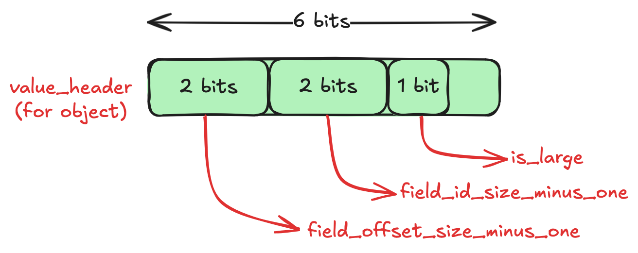
Note that all of this information is packed very tightly. Only using the least number of bits necessary to store it. We have only read 1-byte till now! This is Optimization No. 2.

We will see in a bit how these fields in the header are used. Now that we have the header, we can start decoding the value data.

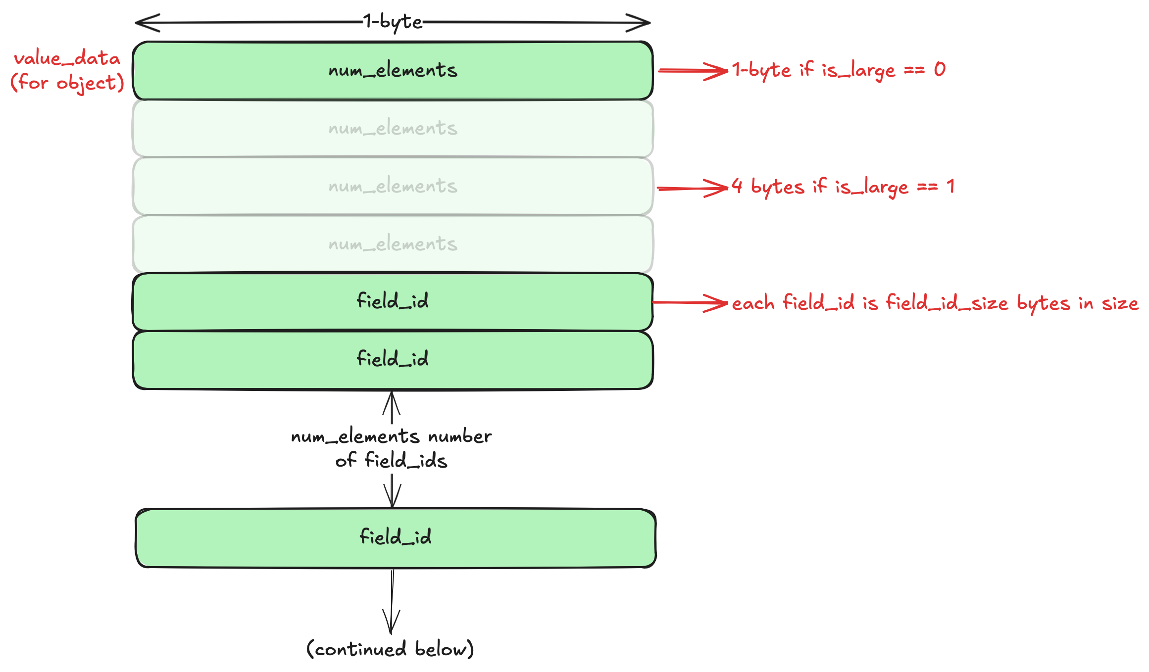
The value_data for object starts with the number of elements (fields). There’s an optimization in the format here for small objects (less than 256 elements). The num_elements is stored in a single byte for small objects, and this is indicated by the is_large field in the value_header. For larger objects, the num_elements is a 4-byte number (which means that we can have a variant object with 4 billion elements!). This is Optimization No. 3.

This is followed by the field_id of each element. These are the keys of the object. But why is this a number and not a string, especially given that JSON objects only have string keys? This is where the metadata binary field comes in. The metadata is a dictionary of all key names in all objects contained in the value. It maps the field_id to the actual key name. Even if the key name appears multiple times in the variant object, we only store it once and refer to it by the field_id. This is Optimization No. 4.
Also, the size of each field_id is not fixed. It depends on the field_id_minus_one field (which is of 2 bits) in the value_header. So we can have 1 to 4 bytes per field_id. This is also an optimization for small objects (objects with <256 unique keys will only need 1 byte). We have Optimization No. 5.

We’re still not done with the object value_data:

The field_ids are followed by the field_offsetss. These are optimized similarly, with each field_offset taking up field_offset_size_minus_one + 1 bytes (this value is obtained from the value_header). We now have Optimization No. 6. Each field_offset is the byte offset of the corresponding value relative to the first byte of the first value. So the 2nd field_offset is the byte offset of the 2nd value and so on. This is needed because each value in a variant object can be of any type, which means each value can be of any size! There’s one extra field_offset that points to the byte after the end of the last value.

One more optimization: the field_ids and the corresponding field_offsets are always sorted in lexicographic order of the actual field names. This means that we can use binary search here! We start at the field_id in the middle and look up the name in the metadata dictionary. Based on the field name, we compare it with the field we’re looking for (in our case users) and move to either the left or the right half. This provides significant improvements for large objects (> 256 objects). We have Optimization No. 7.

The value is where the magic happens. It’s recursive! It starts with a value_metadata (which has basic_type and value_header) again. This property allows the structure to be infinitely nested.

Now that we have the users field, we know it’s an array. Let’s examine the value_header for the array, which has a basic_type of 3 (or 11 in binary).

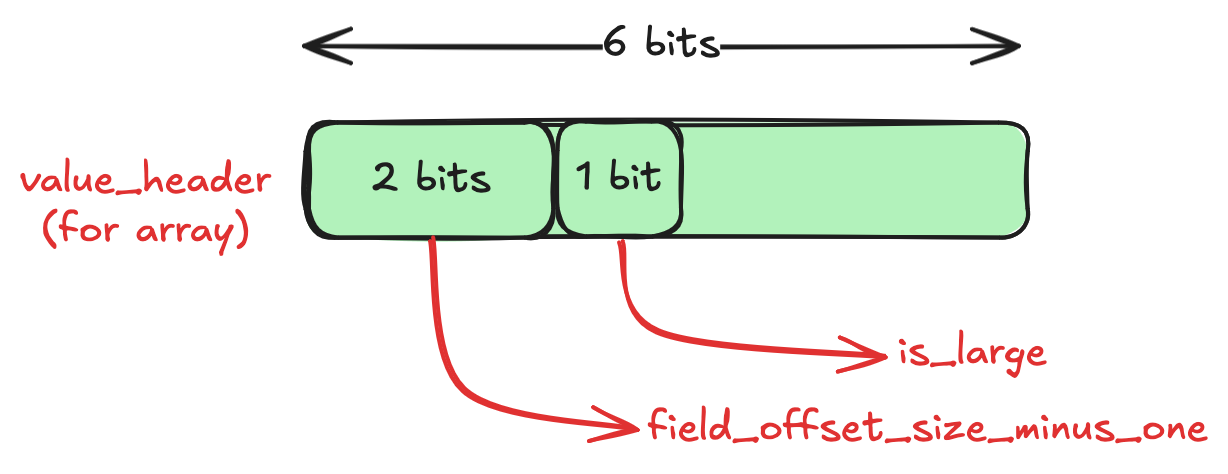
This should look familiar. It’s the same as that of the object, with one less field. Now let’s see the value_data for the array:

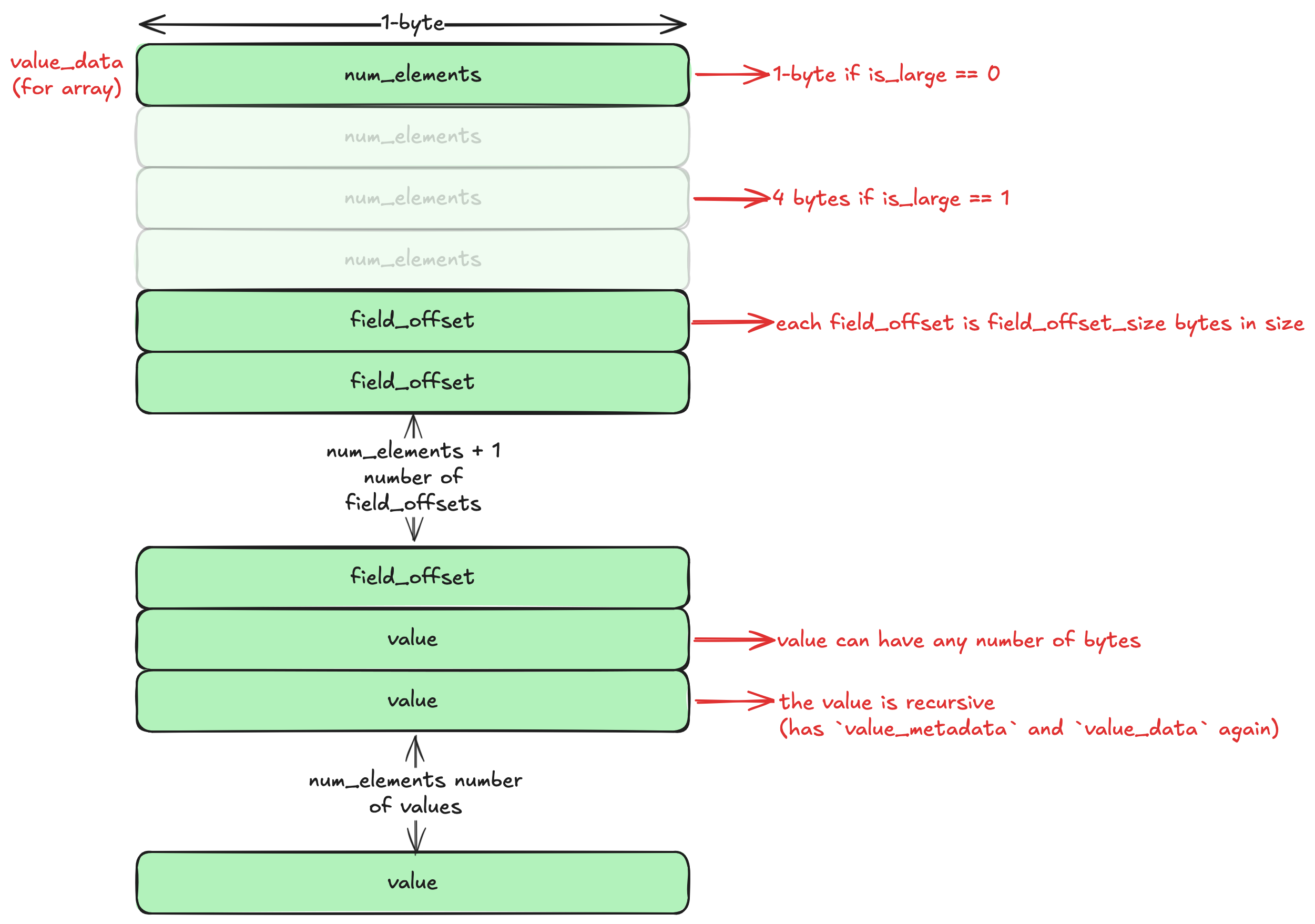
This should also look familiar. We have num_elements number of field_offsets and values. Note that each value is recursive here, too. This means that each element of the array can have a different type: one integer, one string, one object, or even another array.

We have covered users[3] part of the original path users[3].age. We find an object inside the array element and we move our offset to the age field. We know from the query that age is supposed to be an integer field. All primitive values have a basic_type of 0. The value_header encodes a “Type ID”. You can find the full table of primitives here. This extensive list of types enables efficient storage of specific values, using just enough bits to store them. This is Optimization No. 8. For our age field, let’s consider that it’s stored in an int8 type with a Type ID of 3. The value_data of this value contains the 1-byte int8 number.

Consolidating the above 8 optimizations, the JSON String will now look like this in the Variant Binary Encoding:

We now have the exact value we need, without having to parse any of the other fields or array elements. We still need to convert it to an SQL integer - the cast ::int part.

e6data’s query engine is a vectorized one. Data is stored in a columnar manner, even in-memory, in chunks of multiple rows (usually 8192 rows). These chunks of columnar data are called ‘vectors.’ These vectors are similar to those in Apache Arrow. For example, a vector of integers has a similar memory representation to a simple array of integers: it is contiguous in memory, with each element occupying 4 bytes.

With this context, we can now understand the variant implementation. We have a variant vector that stores a chunk of variant values. The value and metadata binary fields are also represented as two binary vectors. Binary vector’s memory representation is similar to that of Apache Arrow’s BinaryArray. This reduces memory fragmentation and increases cache efficiency, since all values in a vector are contiguous. We have Optimization No. 9.

When we perform the JSON path traversal, we keep an additional array of offsets for each row. Once the traversal is complete, we end up with an array of offsets pointing to the exact element we need to extract. Then we simply load the value at each offset into a vector of the specific type (in the case of age field, it’s an int32 vector). This is Optimization No. 10.

This completes the process of reading and extracting values from a variant column. We looked at 10 different optimizations that make this faster than JSON strings.

Variant Data Type Vs. JSON String in SQL

These results show the speed up achieved by variant even on simple queries. The variant column in these queries stores data that looks like this:

{
  "nested_field_name": {
    "nested_field_name": {
      "nested_field_name": {
        ...
            "nested_field_name": {
              "primitive_value" 123
            }
        ...
      }
    }
  }
}

The nesting depth varies per row, with an average depth of 1.46 and a maximum depth of 17 over all 10 million rows. In the first scenario, we are querying just the top-level field in each row, with a query that looks like this:

select count(variant_col:nested_field_name) from variant_type.variant_10m_delta;

In the case of JSON strings, this requires first parsing the whole JSON, extracting the nested_field_name field, and re-serializing the data into JSON. But in the case of Variant, we simply move the offsets of the value binary vector to point to the inner field’s value. The actual buffers are copied directly with a memcpy. This results in a 7x speed up over JSON strings.

For deeply nested access, the overhead of creating the new JSON is lower since those strings are shorter, which is why we see a 3.6x speed up with variant. Keep in mind that our JSON strings implementation has undergone numerous optimizations over the years, whereas the variant implementation is fairly new with quite a bit of scope for more performance optimizations. So the performance of Variant is likely to improve over time compared to JSON strings.

Conclusion and Future Work

We saw how the variant data type helps us achieve significant speed ups in queries over semi-structured data. While the performance is already ahead of JSON Strings, there are a couple of more ideas to improve this even further:

1. Reading the metadata / value binary fields in a German-style binary vector instead of a plain offsets-based binary vector. This is similar to Binary View arrays in Arrow. Using these vectors, we can de-duplicate row values by simply pointing the offsets to a single copy of each unique data. This especially helps in the case of the metadata binary field since field names are not likely change per-row. This reduces memory usage and increases cache efficiency even further.
2. Variant shredding: this is an optimization where frequently accessed nested fields from the main VARIANT binary blob are extracted and stored as their own distinct, top-level columns within the Parquet file. This means that for queries that only touch these “shredded” fields, the performance will be the exact same as normal top-level columns! We also get stats for shredded fields, which enables optimizations like filter pushdown. Shredding is currently being developed as an open standard for both Apache Spark and Delta Lake, and e6data is actively engaged to ensure our engine is ready to support and optimize these powerful advancements as they become available.

‍

‍

‍

‍