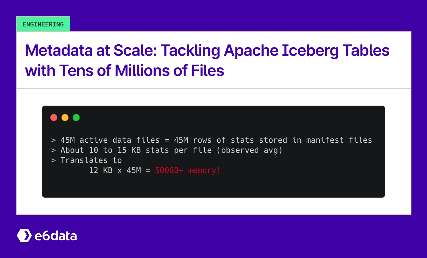
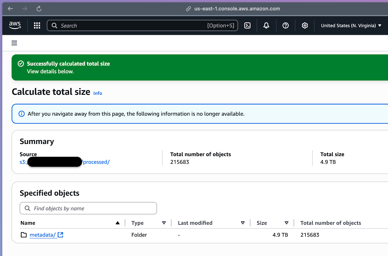
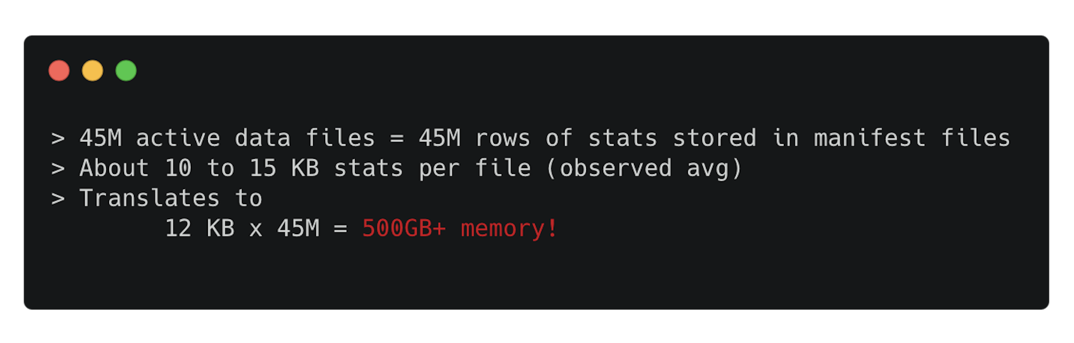
Modern analytic pipelines often focus on dealing with tables with huge data volume, but metadata at scale is an underappreciated threat. Consider a real-world Iceberg table with 45 million data files (~50 TB data). Now, these files produced a 5 TB metadata footprint across ~200,000 files.

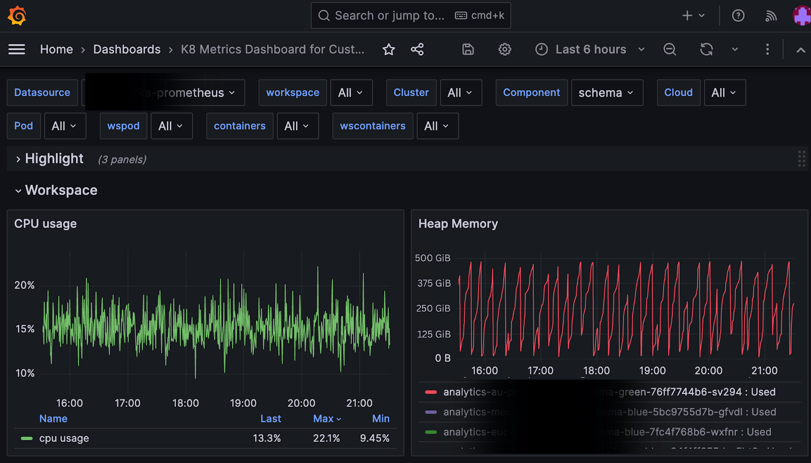
Theoretically, the Iceberg Specifications are designed to plan for large table scans better with the help of a metadata hierarchy. The file size is not the issue; it’s the number of active data files that’s the issue. Planning queries on this table would try to load mountains of file metadata and crash the job. We saw query coordinator nodes OOM (out-of-memory) after reading stats for ~22 million files, entering retry loops, and stalling the entire workload.

Why did this happen? It turns out that file count kills faster than data volume. A wide table (with hundreds of columns) magnified metadata size per file with each data file’s min/max stats, and null counts bloated to 200KB–1MB stats per file, adding up to 5TB of metadata. Even though 50 TB of raw data is manageable, the Iceberg metadata (intended to speed up queries) became the bottleneck. Naively loading all metadata for pruning means materializing millions of records in memory, i.e., a one-way ticket to a crash. We needed to rethink how query engines should handle Iceberg metadata at scale.

This post will dive into three core solutions we implemented to scale Iceberg metadata for real-time analytics:

1. Streaming metadata reads – reading table metadata in bounded chunks instead of all at once.
2. Layered pruning – pruning at multiple levels (partition and file) to drastically cut down the metadata scanned per query.
3. Treating metadata as first-class data – leveraging query engine features (filter pushdown, caching, etc.) by modeling metadata as a queryable dataset.

Along the way, we’ll illustrate with the 45M-file example, highlighting symptoms (e.g., query planning OOMs, long planning times) and the benefits of each approach. I’ll break down how to tame metadata at scale in Apache Iceberg.

Streaming Metadata Reads (Don’t Load Everything at Once)

The first defense against the metadata surge was streaming metadata reads. Instead of loading every manifest and file statistic into memory in one go (a naïve full read that almost guarantees OOM), we stream the metadata in manageable batches. Practically, this means retrieving a subset of manifest files, processing them, then discarding those metadata objects before moving on. By not materializing the full metadata at once, we keep memory usage bounded and predictable.

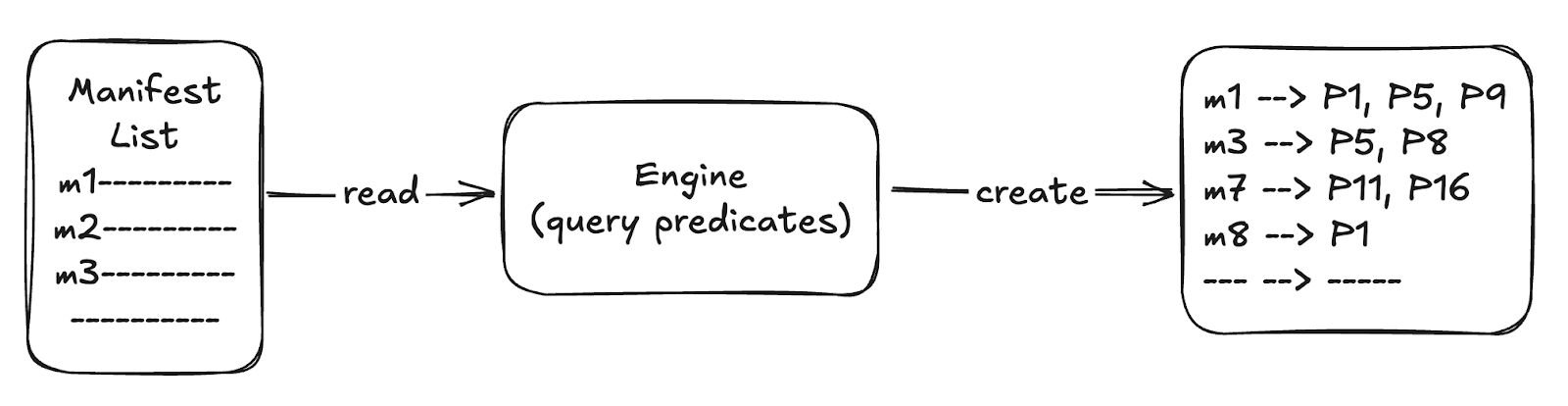
Iceberg’s architecture actually makes this easier. Each Iceberg table snapshot has a manifest list that includes summary stats for every manifest (like partition column’s min/max values and file counts). We use these manifest summaries to decide which manifests are relevant for a given query predicate before reading them. For example, if you query a specific date or partition range, the manifest list tells us which manifest files contain those partitions. We then stream-load only those manifests, a few at a time, instead of grabbing all manifests. Memory consumption is determined by the batch size * concurrency rather than the total metadata size.

The key insight was that we realised we didn’t need to have all the stats in memory at once. This streaming approach meant that even if the table had 5 TB of metadata, the query planner might only ever hold, say, 500 MB or 1 GB of it in memory at once. As soon as one batch’s pruning work is done, we throw those materialized statistics away and load the next chunk. No more single massive memory spike! In our tests, streaming metadata reads eliminated the coordinator OOMs and dramatically improved planning stability. It aligned with Iceberg’s design philosophy too: the spec emphasizes using metadata to avoid expensive file list scans. In short, read metadata in chunks, use it, then free it. This lays the groundwork for the next optimization: layered pruning.

Layered Pruning: Partition and File-Level Pruning

If streaming ensures we don’t choke on too much metadata at once, layered pruning ensures we don’t read unnecessary metadata at all. Iceberg already prunes data files using partition and column stats (min/max). We supercharged this with a two-layer approach:

Layer I: Partition (Manifest File) Pruning

We push down the query filter to the manifest list level, essentially carrying out partition pruning in the metadata before touching any manifest files. The manifest list contains partition summaries for each manifest (e.g., a manifest covers partition date=2023-01-01 through 2023-01-31). We evaluate the query’s WHERE clauses against these summaries to find which manifests could have matching data. All other manifests are skipped entirely; their file stats aren’t even read. This results in avoiding opening tons of manifest files that belong to irrelevant partitions, and we get a list of just the manifest files we do need to read.

In our 45M file example, a selective query might only touch a few hundred manifest files instead of thousands. We also build an optimized mapping of qualifying manifest files to the partitions they contain. This was crucial to organizing the next phase by partition.

Layer II: File Pruning within Manifests

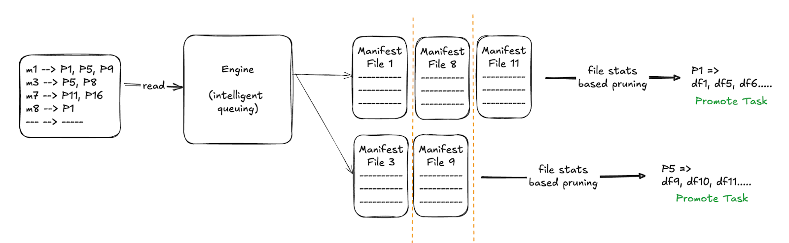
For each manifest file that passed the partition filter, we stream-read it (again, not loading it fully into memory at once) and finally do the data file-pruning using first - the exact partition values and then the column statistics (min/max values, record count, null counts, partition value). Only files that actually match the query conditions get released for scanning. Here we introduced an intelligent queueing: we prioritize reading manifests partition by partition. For instance, if Partition P1’s data is needed, we don’t wait to read all other manifests; we immediately queue up all manifests for P1 and complete their file pruning first. This way, the engine can start processing P1’s actual data sooner, while other partitions’ metadata is still streaming in. It’s like finishing one task completely before others, to unlock parallel execution downstream. Layered pruning at the partition and file level means the query planner deals with far fewer metadata entries overall. We saw significantly faster planning. Instead of scanning 45 million entries, a query might only scan a few hundred that survive both pruning layers.

Benefits: Layered pruning slashes unnecessary work. By cutting out whole manifests upfront, we reduce I/O and CPU spent deserializing metadata. By pruning file entries, we further trim the in-memory planning dataset. Our partition pruning step addresses that by leveraging Iceberg’s manifest-list partition stats to skip entire manifests that have no matching data. Together, streaming + layered pruning turned minutes-long planning (or failing queries) into sub-second planning for many cases. It also kept memory usage low and predictable, preventing the planner from ever attempting to load the full 5 TB again.

Treating Metadata as First-Class Data

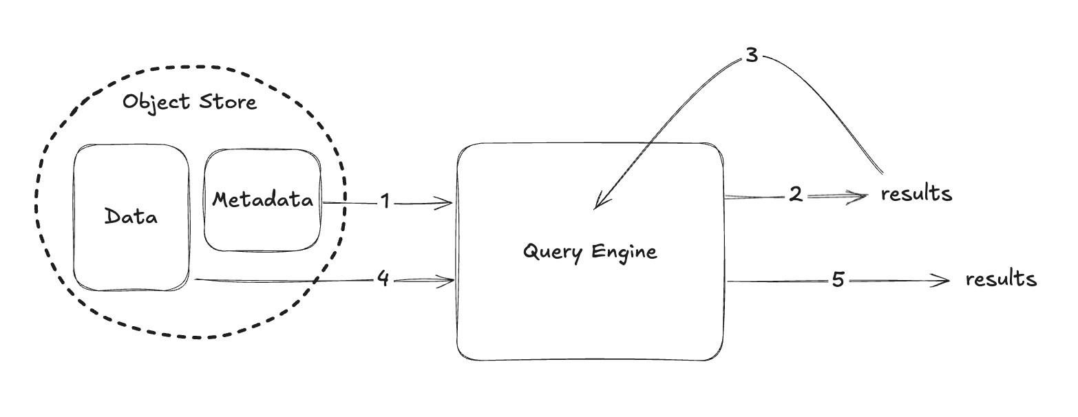
Perhaps the most powerful shift was to start treating metadata itself as a first-class dataset. In other words, we made our query engine query the metadata using SQL before querying the actual data. We adopted a two-query pattern: when a user submits a SQL query on the table, the engine breaks it into Query 1: a metadata query and Query 2: the original data query. The metadata query can be as simple as “SELECT file_path FROM table.files WHERE <predicate on partitions or stats>”. This returns the list of data files that actually contain relevant data, using only metadata. Then, Query 2 reads only those files. By doing this, we prune out empty or irrelevant data files using pure metadata with all the power of SQL optimizations that we have built for data.

But why go to this trouble? Because once we model metadata as a table, we unlock the full arsenal of query engine optimizations without writing custom code. The engine can apply projection pushdown (reading only the few columns needed, e.g., just file paths and maybe min/max of one column, instead of all stats) and predicate pushdown at the metadata scanning stage. We can cache frequently used metadata slices in memory or on disk, just like caching a query result. We plan metadata reads with full parallelism and distribution; for example, many threads or workers can scan different manifests concurrently, just as they would scan data partitions. Essentially, we treat the Iceberg manifest/metadata layer as another workload to optimize.

This approach also revealed the missed opportunities in naive streaming: some manifest files might contain zero rows matching the query, but if you stream them fully and check row by row, you waste effort. By pushing filters down and skipping entire manifests early (manifest-level skipping), we avoid reading those altogether - similar to partition pruning but based on file stats content. We even extended this concept with materialized views and indexes on metadata. For instance, we could maintain a smaller derived table of just “partition -> list of manifests” or use Bloom filters on high-cardinality columns in the metadata to quickly test if any file might contain a value. By using metadata as data, any improvement to the query engine or new optimization (say a better cache or a new index type) automatically benefits metadata retrieval as well, future-proofing our solution.

In practice, treating metadata as first-class data meant our engine could handle tables with tens of millions of files gracefully. Planning operations that previously tried to cram 5 TB of stats into memory now behave like running two lightweight queries: one that quickly filters down file candidates, and one that scans the minimal necessary data. It reinforces the idea that metadata is a valuable dataset in its own right and not an overhead. When used wisely, it speeds up query planning instead of dragging it down.

Example Scenario: 45M Files and an OOM Nightmare (and Fix)

To crystallize these concepts, let’s recap the 45M-file table scenario. The table had ~50 TB of data split into 45 million small Parquet files (thanks to append-heavy streaming ingestion). The Iceberg metadata ballooned to ~5 TB across 200k manifests, because each file’s stats were ~0.2–1 MB (a wide table with ~300 columns, each file’s min/max stats occupied significant space). A simple analytical query (e.g., a sum over a month of data) would crash the Spark or Trino planner and then fail with a Java heap OOM as it attempted to read the entire metadata set for pruning. The logs showed the planner reading millions of file entries, then dying mid-way. Even when it failed at ~22 million files in, the query engine would retry, often looping fruitlessly while holding cluster resources hostage. Other queries slowed down because the catalog service was busy thrashing on this one. This is the hallmark of a metadata bottleneck: the planning phase takes so long that the cluster can’t even start executing the actual data scan.

After implementing our three-step solution, the outcome was a complete transformation. Streaming reads ensured the planner only used a fixed chunk of memory (no more monolithic 5 TB loads). Layered pruning ensured perhaps over 95% of manifest files never even got touched for a given query (e.g., if the query was for one month, only that month’s partitions’ manifests were read). Treating metadata as data lets us push down filters and only pull back, say, a few thousand matching file paths out of 45 million. The query that previously crashed now plans in seconds and executes successfully. We effectively taught the query engine to respect the metadata using pruning and streaming instead of brute force. A huge number of tiny files or extremely wide tables can make metadata the dominant factor in cost in terms of latency as well as memory, if not handled properly.

Conclusion

In summary, scaling Apache Iceberg metadata requires rethinking how we read and use table metadata. Here are the key takeaways:

• File Count Matters More Than Data Size: A million 5MB files is often worse than a few 5GB files. Too many small files lead to bloated metadata (manifests) and slow planning. Monitor tables where metadata size approaches or exceeds data size.
• Stream, Don’t Chug: Avoid loading all metadata in one shot. Stream your metadata reads in chunks to keep memory usage O(constant). This prevents OOMs and keeps query planning robust even as tables grow.
• Prune at Multiple Layers: Push filters down to the manifest list to skip whole partitions/manifests, and then prune at the file level using stats. Narrow the search space early and aggressively; it cuts query planning time and work by orders of magnitude.
• Leverage Metadata as Data: Treat Iceberg metadata as a queryable dataset. Use metadata tables or a two-step query plan to apply predicate pushdown, projection, caching, and indexing on metadata. This unlocks advanced optimizations (like Bloom filters and materialized views on metadata) and reuses existing query engine smarts for planning.
• Metadata Isn’t Just Overhead: Ultimately, metadata can be your asset if you know how to use it. Well-designed metadata handling turns Iceberg’s rich metadata into a speed-up feature rather than a bottleneck.

By implementing these strategies, you can ensure their Iceberg tables remain query-optimized and robust, even with tens of millions of files and terabytes of metadata.