In the last post of our Vector Search Blog Series, Vector Search in the Lakehouse: Unlocking Unstructured Data, we introduced how text embeddings can turbocharge search by capturing semantic meaning, allowing SQL queries to find results by concept rather than exact keywords. Now, let’s dive deeper into the practical details behind that approach. We’ll go through some SQL examples using cosine similarity, compare a few popular embedding models (MiniLM, SciBERT, CodeBERT) and their characteristics, outline how e6data uses LOAD VECTOR to generate embeddings, and share guidance on choosing cosine similarity thresholds for semantic search.

Searching with Cosine Similarity in SQL (Before and After)

One of the biggest benefits of vector embeddings is the ability to perform similarity search in SQL using cosine similarity (or distance) metrics. The earlier blog in the series had a simple example using an Amazon product reviews dataset. Let’s use the same example again. Suppose we want to find reviews with headlines semantically similar to the phrase “amazingly good.”

Before (Keyword Search): Originally, we might have used a keyword filter like this:

SELECT review_id, review_headline 
FROM reviews 
WHERE review_headline ILIKE '%amazingly good%';

This would return only rows where the exact words “amazingly good” appear in the headline, missing out on tons of phrasing variations. In fact, running a query like the above will only fetch a handful of hits and miss tens of thousands of paraphrases expressed in different words. However, if keyword search is powered by text indexing solutions like BM25 indices, users can carry out searches that can be a synonym or a partial match.

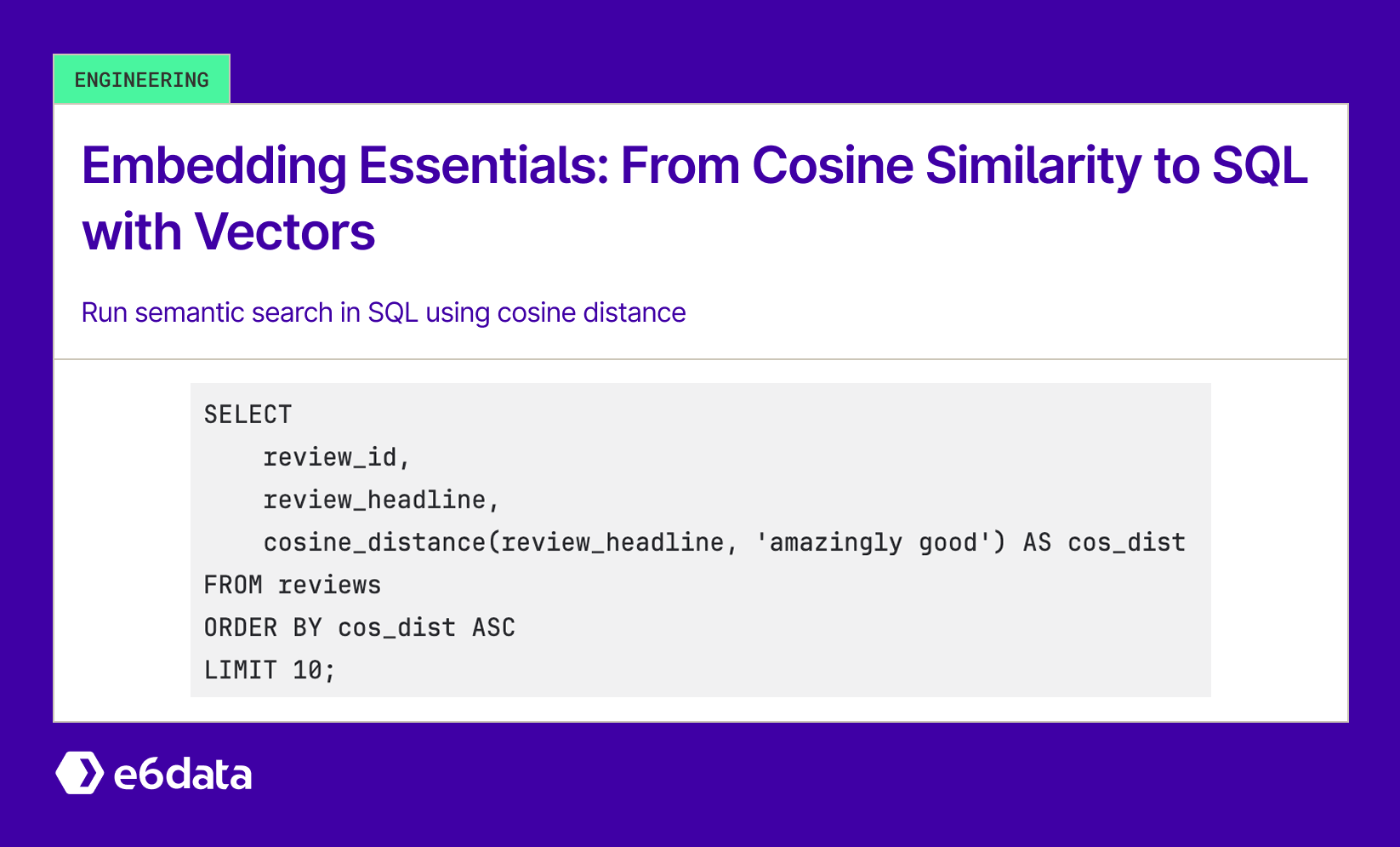
After (Vector Similarity Search): e6data tries to keep vector embeddings transparent to the search operation, so the end user would query the column as if it were a predicate on the raw text, but e6data understands that it is a vector search operation and delegates the lookup to the underlying embeddings automatically. At runtime, the engine derives an embedding for review_headline on demand, so the SQL remains focused on the original column while the vector math happens underneath. A query to retrieve reviews semantically close to “amazingly good,” therefore looks like this:

SELECT
    review_id,
    review_headline,
    cosine_distance(review_headline, 'amazingly good') AS cos_dist
FROM reviews
ORDER BY cos_dist ASC
LIMIT 10;

Here, cosine_distance(review_headline, 'amazingly good') computes the cosine distance between the review’s headline embedding and the embedding of the phrase “amazingly good”. The results are ordered by cos_dist ascending (i.e., most similar first). The query performs a nearest-neighbor search in embedding space, surfacing semantically related reviews even when they don’t share the literal words, for example, “absolutely fantastic purchase” or “really good quality.” Any headline conveying a sentiment similar to “amazingly good” moves to the top.

Comparing the before and after queries makes the advantage pretty clear. The “before” version depended on literal string matching; the “after” taps directly into the embedding space while preserving the familiar column names. We get significantly improved recall of relevant results without changing our schema or query style.

Comparing Embedding Models: MiniLM Vs. SciBERT Vs. CodeBERT

Not all embeddings are created equal. Let’s compare three pre-trained models for generating vectors, highlighting their dimensions, speed (latency), and domain suitability:

‍

• MiniLM (specifically the all-MiniLM-L6-v2 model) produces 384-dimensional embeddings. It’s a distilled 6-layer model, so it’s much smaller and faster to run. In tests, MiniLM’s low latency means you can embed text quickly, making it ideal for interactive queries or frequent batch updates. The trade-off is slightly lower accuracy on nuanced semantics compared to larger models, but for many general-domain tasks, it was still very good. MiniLM is excellent as a default because it offers 5x faster embedding generation than a full-size BERT model while retaining a lot of semantic fidelity.
• SciBERT is based on the BERT architecture but trained on scientific literature. It outputs 768-dimensional vectors, double the size of MiniLM’s. SciBERT tends to be slower (given its larger network and output size), but it really shines if your text is scientific or technical (e.g., research paper abstracts, medical text). In domain-specific evaluations, SciBERT captures jargon and domain-specific nuances that a general model might miss. The extra dimensionality potentially allows it to encode more information relevant to science content. However, if you use SciBERT on everyday user reviews or general text, you might not see a huge gain. So, it’s ideal to choose SciBERT only when domain specificity is crucial.
• CodeBERT is another 768-dimension model, originally a RoBERTa-based model trained on natural language and code. This was included to experiment with embedding software-related text (like code snippets or Stack Overflow posts). As expected, CodeBERT is geared towards code and technical domains. Its performance on plain English reviews was fine (comparable to a BERT), but not better than MiniLM for our use case. It is also as slow as SciBERT due to similar size. If you’re looking to build a semantic search for a programming knowledge base or doing code-to-code search, CodeBERT would be a top choice. But for product reviews, it doesn’t offer an advantage over the others.

How We Generate Vector Embeddings

With a model selected (MiniLM for its speed, SciBERT for scientific nuance, or CodeBERT when we’re embedding code), the next step is to turn raw text into vectors inside the lakehouse. That hand-off from “which model” to “how we generate and store” is handled by this command.

LOAD VECTOR INTO reviews(review_headline);

When this statement runs, the engine performs a parallel scan of reviews. For each headline, it calls the text-embedding service you chose. The command never writes an _embedding column back to the table; instead, it emits vector files in a purpose-built storage format we call Blitz.

Why Blitz?

Blitz stores vectors contiguously, with an offset table that supports O(1) lookup. During ingestion, we also apply scalar quantization, where 8-bit integers replace 32-bit floats, shrinking each 768-dimension vector from roughly 3 KB to about 0.75 KB. Quantization is lossy, but it preserves enough angular information for a coarse search and dramatically improves cache locality.

After vectors are on disk, every similarity query follows a two-pass plan:

1. Pass 1 – Quantized scan
   The search kernel compares the query vector (also quantized on the fly) against all Blitz blocks, using fast integer dot products. This pass prunes the candidate set by orders of magnitude.
2. Pass 2 – Full-precision rerank
   Surviving row IDs retrieve their original float32 vectors (still stored in Blitz), and the engine recomputes cosine similarity at full precision to produce the final ranking.

Because quantized data are an eighth the size of the originals, Pass 1 is memory and I/O-friendly. Pass 2 touches only a tiny fraction of vectors, so the cost of full precision is negligible. The overall effect is sub-second search over millions of rows without maintaining a separate vector database; the vectors live in the lakehouse, managed by the same transactional metadata as the base table.

Choosing the Right Cosine Similarity Threshold

One often asked question is: What cosine similarity (or distance) threshold should I use for filtering results? We used a threshold in the WHERE clause (e.g., cosine_distance(...) < 0.1) to only return close matches. Picking this threshold required a bit of tuning and understanding of the embedding space.

Here’s an experience of adjusting the threshold from 0.2 to 0.1 and its impact:

• At first, we tried a cosine distance <0.2 (which corresponds to cosine similarity ≈ 0.8 or higher). This yielded more results, i.e., it cast a wider net for what was considered “similar.” However, looking at the output, some matches were only tangentially related. A distance of 0.2 allowed somewhat loosely similar items to sneak in. For example, a query for “refund frustration” might bring back a review about “delayed shipping,” which is a bit off-topic, just because the model found some mild semantic link.
• We tightened the threshold to cosine distance <0.1 (cosine similarity ≈ 0.9+). Now the results were much more precise (mostly very relevant hits) but, of course, fewer in number. Using the 0.1 cutoff for “too expensive” or “amazingly good” queries meant only reviews that were almost verbatim in sentiment would show up. This is great for precision, but you risk missing some valid paraphrases that are just worded differently.

The “sweet spot” depends on your application’s needs. We suggest an approach to find this: “visualize the distribution” of cosine similarities between your query (or a set of example queries) and a large sample of data. In practice, we took a random sample of pairwise cosine distances and plotted a histogram. What we saw was a sort of bimodal or skewed distribution; many pairs were dissimilar (distance closer to 1), and a smaller cluster was highly similar (distance near 0). This helps inform a threshold: you might see a “gap” or elbow in the distribution where similar vs. dissimilar items separate.

We also validated against known pairs to choose the threshold. In our case, we had some known duplicate or equivalent phrases in the data. For example, we knew “didn’t meet expectations” should match “want my money back” (both indicating refund requests), whereas “arrived late” should not match “not worth the price.” We checked the cosine distances for these known examples: the similar pair had a distance around 0.05, and the unrelated pair was around 0.3. This gave confidence that setting a cutoff around 0.1 or 0.15 would include the good pair and exclude the bad one. Essentially, we confirmed the threshold with a few examples.

Our guidance on thresholds is: start with something somewhat strict (like 0.1 for distance, i.e., 90% similarity) and then adjust if you feel you’re missing too many results. If you retrieve too few hits, loosen it (0.2 or even higher). If you see off-target results, tighten it. The distribution plot and sample pairs method can greatly accelerate this tuning by giving you a sense of typical distances in your dataset. Every model and dataset will behave a bit differently (for instance, a model might generally produce tighter clusters vs. spread-out embeddings), so there’s no one-size-fits-all number. Threshold tuning is an iterative process. It’s worth spending time on because it directly affects the quality of your semantic search results.

Finally, remember that you don’t always need a hard cutoff. Sometimes, you might sort by similarity and just take the top K results instead of thresholding absolute values. We did this in some of our demo queries (just ordering by cos_dist and limiting to 10 or 50 results). This way, you always get some results back, ranked by relevance. A threshold is more useful when you want to say “only show very similar matches or nothing.” In a production setting, we might use a combination: e.g., take the top 50 but also drop anything with a distance above 0.3 as a sanity filter.

Final Thoughts

By enriching SQL with vector search capabilities, we bridge the gap between unstructured text and structured queries. In this deep dive, we expanded on how exactly we implement and fine-tune such a system: from writing SQL queries using cosine_distance for semantic matching, to weighing different embedding models for quality vs. speed, to building a robust pipeline that generates and stores embeddings in our lakehouse, and finally to tuning similarity thresholds that yield relevant results. All these details come directly from our project’s journey, and we hope they help you in your own implementation.

The key takeaway is that working with embeddings in SQL is not only feasible, it’s incredibly powerful. With the right model and careful engineering, you can unlock new insights from text data within your familiar data warehouse or lakehouse environment. And as always, the journey is iterative: test, visualize, and tune as you integrate vector search into your applications.

‍

‍

‍

‍