How to Optimize Snowflake Queries for Enterprise Data Teams? {2025 Updated Guide}
August 14, 2025
/
e6data Team
Snowflake
Query Optimization
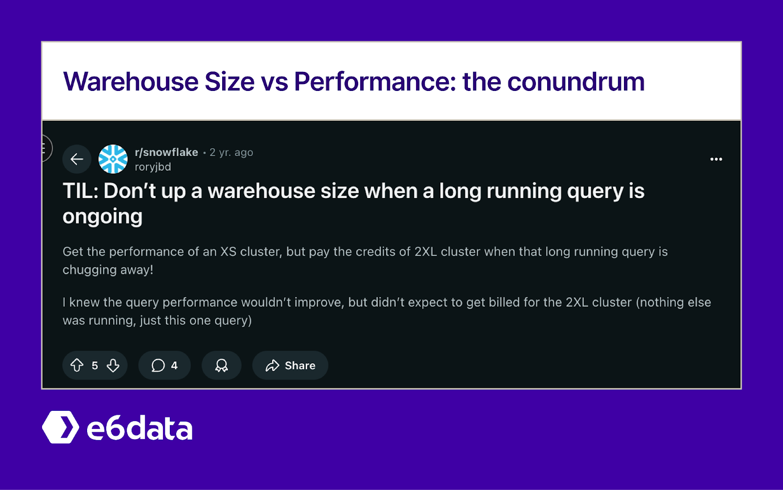
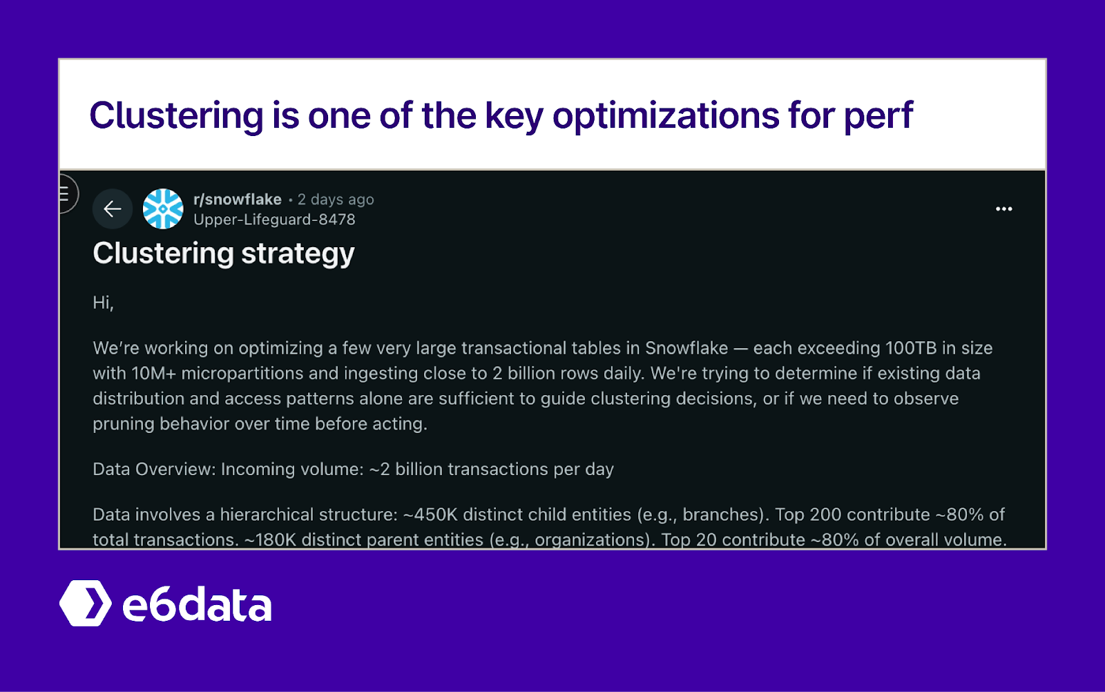
Redditors discuss query optimisation in Snowflake warehouses
Snowflake might be a powerhouse out of the box, but letting it run “as-is” can burn money and time. Any data platform, even Snowflake, will underperform if misused. This guide cuts past the fluff and typical doc-speak to deliver sharp, opinionated advice on squeezing maximum performance (and value) out of Snowflake. The goal is simple: make your queries faster and your credits go further. We’ll cover everything from sizing warehouses smartly to reading query profiles, with real-world examples and direct recommendations. No vague platitudes – just actionable techniques that enterprise architects and Snowflake customers can apply today for immediate impact.
Slow dashboards erode trust. View 90th-percentile runtimes in Query History.
Partition-pruning ratio
Scans > 50 % of partitions
Low pruning means reading unnecessary data. Compare “Partitions scanned vs total” in Query Profile.
Disk spillage
Any spill to remote storage
Spills slow queries ~10×. Look for “Bytes spilled to remote” in Query Profile.
Heavy-hitter queries
Single query/user > 30 % daily credits
One rogue query can blow the budget. Use Resource Usage views to find hogs.
Serverless burst pattern
Many micro-queries with long idle gaps
Compute spins up/down too often. Check WAREHOUSE_START_STOP _HISTORY for churn.
Warehouse Sizing: Bigger Isn’t Always Better
Choosing the right warehouse size is not about picking the biggest and hoping for the best. In fact, oversizing warehouses is a common rookie mistake that leads to wasted credits. Warehouse “right-sizing” means matching compute power to your workload’s needs:
Warehouse Size vs Performance: the tradeoff
Start Small, Scale as Needed: Don’t jump straight to an XXL warehouse “just in case.” Snowflake bills per second, so a larger warehouse used briefly might cost less or more, depending on usage. Benchmark on a smaller size first, then scale up if the query truly needs it. Remember, one hour on a 5XL can cost more than 10 hours on an XS – so using a giant warehouse for a quick task is often overkill. Conversely, if a job can finish in 10 minutes on a 2XL instead of 60 minutes on a Small, the larger size might actually be cheaper overall. Test and find the sweet spot.
Watch Concurrency and Queuing: High user or query concurrency can choke a small warehouse. If you regularly see more than 5–10 queries running at once or queries queuing, it’s a sign that the warehouse is too small. In Snowflake’s History or Warehouse Monitor, check if queries spend time in a “Queued” state – if yes, consider a bigger size or scaling out.
Use Multi-Cluster for Spikes: Rather than running an oversized warehouse 24/7, use Snowflake’s multi-cluster warehouses for bursty periods. This feature spins up extra compute clusters automatically to handle concurrency spikes, then shuts them off when load subsides. For example, set MIN_CLUSTER_COUNT = 1, MAX_CLUSTER_COUNT = 3 on a busy BI warehouse, so it normally runs as one Medium, but can temporarily scale out to 3 M-sized clusters during the 9 AM rush. This handles peak load without you manually resizing or paying for an XL all day. (Note: Multi-cluster requires Enterprise edition.)
Isolate Workloads: Don’t mix a heavy ETL job and a BI dashboard on the same warehouse. That’s asking for contention and unpredictable performance. Instead, split workloads by warehouse (e.g., a dedicated “ETL_WH” for batch jobs and “BI_WH” for reports). This way, you can size and tune each warehouse independently, and a nightly load won’t slow down user queries.
Manage Idle Time: A warehouse running but doing nothing is pure waste. Snowflake’s usage views let you check “warehouse idle ratio” – e.g., if a warehouse ran for 12 hours but only did 1 hour of work, you paid 11 hours for nothing. Adjust auto-suspend settings so compute turns off when not needed (e.g., suspend after a few minutes of idle). However, avoid suspending too aggressively during active periods – more on that in the caching section. The balance: don’t pay for idle compute beyond what’s needed to keep things responsive.
Real-world example:
One team had a Medium warehouse running all day just “in case,” but only using ~10% of its capacity most hours. By shortening the auto-suspend to 5 minutes and using a Small for low-traffic times, they reduced their compute bill by 40% without impacting users. On the flip side, another team tried to run everything on an XS to save money – and saw queries queue constantly. Bumping that workload to a Small eliminated queuing and actually reduced overall runtime (and cost per query) because jobs finished faster.
The lesson: right-size each warehouse based on actual usage patterns, and take advantage of Snowflake’s elasticity (scale-out and scale-up) rather than one-size-fits-all.
Cost Modeling: Every Query Has a Price Tag
In Snowflake, performance and cost go hand-in-hand. Every query you run consumes credits, so slow or inefficient queries literally burn money while you wait. Cost modeling is about understanding where your credits are going and aligning them with business value:
Always check your cost per query in Snowflake
Measure Credit Usage Per Workload:Snowflake’s Account Usage schema provides views like WAREHOUSE_METERING_HISTORY and QUERY_HISTORY that expose credit consumption by warehouse, user, query, etc. Use these to identify “heavy hitters.” For example, you might find that one ETL job or one analyst’s queries are consuming 30% of your daily credits. Once you know that, you can dive in and optimize those expensive workloads first. If one report is eating up a disproportionate chunk of credits, tune it or move it to its own warehouse.
Attribution via Query Tags: A pro tip for enterprise teams is to use QUERY_TAG to label queries by project or team (e.g. ALTER SESSION SET QUERY_TAG='finance_etl';). These tags show up in ACCOUNT_USAGE.QUERY_HISTORY, so you can aggregate cost by department or pipeline. This makes it clear which teams or features are driving the bills – fostering accountability and enabling charge-back models if needed. (However boring and redundant it may seem as a practice.)
Cost vs Performance Trade-offs: Model different scenarios for your workloads. How much does it cost to run a given job on a Large warehouse for 10 minutes versus a Medium warehouse for 20 minutes? The credit cost might be roughly equal, but if the Large finishes the job well within your SLA, you might prefer the cheaper Medium even if it runs longer. Or vice-versa: if an interactive query is slow on a Small, running it on a Medium might double the cost but deliver results in seconds instead of minutes, which could be worth it for user productivity. The key is to quantify these decisions. Don’t assume – actually calculate credits consumed in each case (Snowflake’s history will tell you the credits for each run). This analytical approach ensures you spend where it counts and save where you can.
Show the Cost of “Just in Case”: Idle or redundant processing adds up. If a dashboard refresh runs every hour “just in case someone looks at it,” compute how much that costs per week. You might be shocked. Perhaps caching or on-demand execution could save thousands. Similarly, if someone insists on using SELECT * on a huge table for convenience, show them how that single unfiltered query scanned 500 GB and cost several dollars in credits. Tying usage to dollars (or your currency) is a powerful motivator for more efficient queries. Make cost part of the conversation in design and code review – every query has a price tag.
Resource Monitors: Guardrails to Prevent Runaway Spend
Even with good sizing and cost awareness, you want safety nets. Resource Monitors in Snowflake are like circuit breakers for your credit usage. They track consumption and can take action (like send alerts or halt warehouses) when a threshold is reached. In an enterprise setting, this is crucial for preventing unexpected budget blowouts:
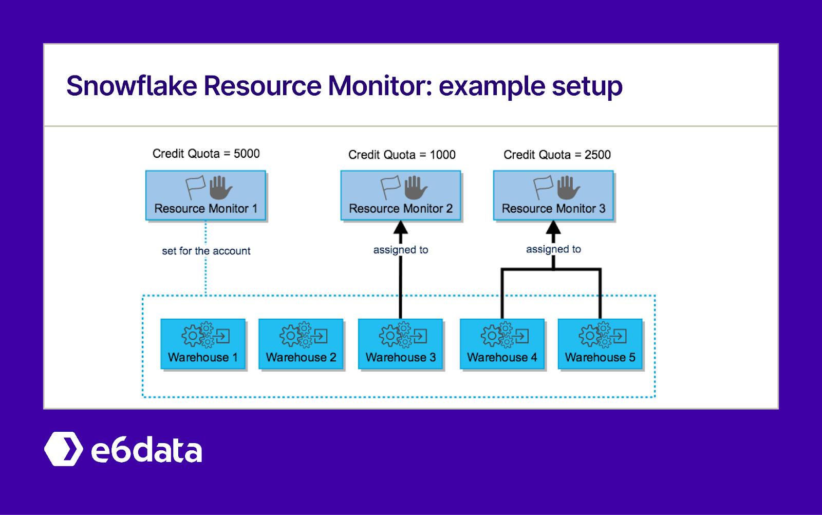
Snowflake Resource Monitor: an example setup
Set Monthly/Weekly Credit Quotas: Define resource monitors to cover your critical warehouses or the whole account. For example, you might set a monitor on your ETL warehouse to notify at 75% of the monthly budget and suspend the warehouse at 90%. This way, if a pipeline goes haywire or someone starts an ad-hoc query binge, you get alerted before costs explode. Attaching the monitor to the warehouse ensures it will automatically pause compute if things go past the hard limit.
Use Suspend Actions Wisely: Monitors can either just notify or actually suspend warehouses. A common pattern is to use notify for prod warehouses (so the team is warned to take action) and suspend for non-critical or dev warehouses (to hard-stop any abuse). For instance, you might allow a marketing warehouse to use up to 100 credits a day and then suspend, preventing any rogue queries from going further.
Pair with Auto-Suspend Settings: A monitor is your last line of defense. In practice, you should also have sane auto-suspend on warehouses (don’t let them idle for hours) and possibly statement timeouts. Snowflake allows setting a STATEMENT_TIMEOUT_IN_SECONDS for a warehouse or account – e.g., cancel any query running over 30 minutes. This prevents a forgotten Cartesian join from running for 5 hours and racking up credits. Think of it as an automatic kill switch for runaway queries. Use these features together: short suspend intervals for idle warehouses, timeouts for long queries, and monitors for overall spend limits.
Review and Adjust: Monitor thresholds shouldn’t be static. Revisit them each quarter or whenever your usage pattern changes (new projects, more data, etc.). If you’re consistently hitting 80% of your monthly quota by mid-month, maybe increase the quota and investigate why usage spiked. The goal of monitors is not just to cap usage but to spark conversations about why a workload is consuming so much. They provide concrete data to drive optimization efforts.
In summary, resource monitors and related controls are your insurance policy. They won’t replace proactive optimization, but they’ll save your bacon if something slips through. No one wants a surprise six-figure cloud bill – set up monitors and you’ll sleep easier.
Cache Usage: Exploit Snowflake’s Free Speed
Snowflake’s architecture offers two key caching layers, and using them well is one of the easiest wins for query performance:
Caching is your best friend for query performance
Result Cache (Zero-Cost Replays): Snowflake has a global result cache that instantly returns the results of a previous query if the same query (text and parameters) is run again within 24 hours. This comes at no warehouse cost – the query doesn’t even hit your compute. For dashboards and repetitive queries, the result cache is gold. It means if five users run the same “sales last week” report, the first run might take 5 seconds, but the next four returns are milliseconds, with zero credits used.
To leverage this, ensure your queries are identical on repeats. Avoid non-deterministic functions like CURRENT_TIMESTAMP in SQL text, which change each execution and bypass the cache. If you need rolling time windows, use constants or date functions that resolve to the same value for a given run (e.g., CURRENT_DATE for “today,” which stays constant during the day). Many BI tools let you parameterize queries such that the SQL text remains consistent – use that feature. Bottom line: cache hits = sub-second response and $0 cost. Design your frequent queries to hit that result cache whenever possible.
Local Disk Cache (Warehouse Data Cache): When a warehouse is running, it caches table data in SSD and memory. If the same data is queried again soon after, Snowflake can read it locally instead of from the remote storage, which is much faster. However, if you suspend the warehouse, that local cache may be dropped. This leads to the infamous “cold start” problem: the first query after resume has to fetch a lot of data from S3, incurring a delay.
The advice: for frequent query workloads (like BI dashboards during business hours), don’t auto-suspend the warehouse too aggressively. Keeping a warehouse warm for an extra 10-15 minutes of idle time can ensure the cache stays hot, so the next query is fast. For example, if your dashboard refreshes every 5 minutes, set auto-suspend to ~15 minutes. Yes, you’ll pay a bit for idle time, but you’ll avoid making every query re-read from storage. It’s a trade-off between a few extra credits versus consistently snappy performance. Many teams find that preventing cold starts is worth it for user experience. If shutting down is necessary (e.g., overnight), consider a scheduled “warm-up” query in the morning (touching key tables) to preload the cache before users hit the system.
Takeaway:Cache is your friend. Use the result cache aggressively – it’s basically free performance. And manage your warehouse caching wisely – don’t penny-pinch on a few idle minutes if it means your users suffer cold-start slowness. In Snowflake, smart use of cache separates the well-tuned deployments from the rest.
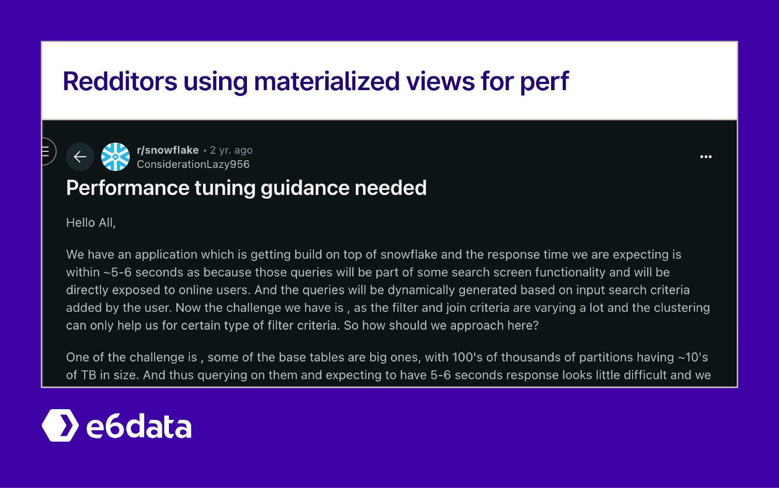
Result Materialization: Precompute Heavy Results for Reuse
Sometimes, caching alone isn’t enough – especially when queries are complex, long-running, or slightly different each time. This is where materializing results can save the day. The idea is to do expensive work once, store the result, and reuse it rather than recalculating repeatedly.
Using Materialized Views in Snowflake for performance
Use Materialized Views for Aggregations: If your analysts or BI dashboards are constantly computing the same aggregate (say, total sales by region by day) over a huge table, consider creating a materialized view that pre-aggregates that metric. Snowflake will maintain the view as underlying data changes. Then queries can simply SELECT * from the materialized view (or filter on it) and avoid scanning the entire base table each time. Materialized views are especially useful for common filtering or joining expensive patterns. Just be cautious: maintaining a materialized view has a cost (Snowflake updates it on data load), so use them for truly frequently-used computations, not one-offs.
Build Summary Tables or Stage Results: In cases where materialized views aren’t a fit (maybe the transformation is too complex or you want more control), you can create your own summary tables. For example, run a nightly job that populates a “last 7 days sales” table. Your dashboard can then simply query this small summary table rather than crunching millions of rows live. Similarly, if you have a query that joins multiple large tables and is used by many users, you might run it once and store the result in a temporary table that others can query. This is essentially manual caching – trading some storage and ETL time to save compute on repeated work.
Use CTAS for Intermediate Results in ETL: For heavy ETL pipelines, don’t be afraid to break complex transformations into steps and materialize intermediate results (using “CREATE TABLE AS SELECT” or temporary tables). For instance, if you have a monster SQL statement with many subqueries/joins, it might be faster and easier to maintain if you break it into parts: generate an intermediate result, index or cluster it if needed, then join to it in the next step. This can reduce duplicate scanning of the same source data across pipeline runs. It can also aid debugging. The trade-off is extra storage and a slightly more complex pipeline, but the performance gains can be worth it.
When Queries Differ, Share the Heavy Lifting: Often, dashboards have slight variations of a query (e.g., the same base data filtered by region or product). Those won’t hit the result cache (different text), but you can design so that they at least use a common materialized result. For example, one query shows “sales by region” and another “sales by product”. Both could draw from a single precomputed “sales by region by product by day” table, each just applying a different filter. The core heavy lifting (scanning all sales transactions) happens once daily to populate that table, rather than for every user query.
In short, identify repeated heavy workloads and consider precomputing them. Snowflake’s compute is cheap when used wisely, but doing the same expensive calculation ten times is just a waste. Save your credits (and time) by doing it once and leveraging the results many times.
Reading Query Profiles: Let the Data Lead You
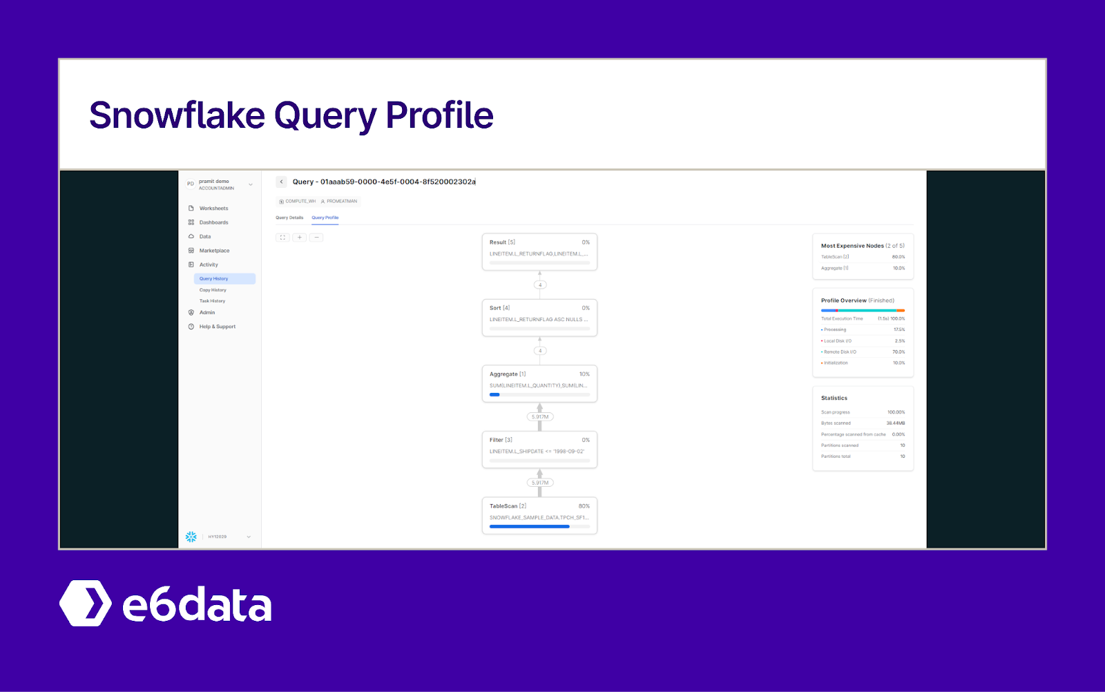
When a query is slow or costly, don’t guess at the cause – Snowflake will tell you if you know where to look. The Query Profile (available for any executed query in the UI) is an invaluable tool to diagnose performance issues. It’s your per-query X-ray, showing how the query executed and where time was spent.
Snowflake Query Profile interface
Here’s how to use it:
Check Scan vs Prune: One of the first things to look at is the micro-partitions scanned. The profile shows “partitions scanned” out of total. If your query scanned 500 out of 500 partitions of a table (100% of the data), that’s a red flag. It means no pruning was happening – perhaps your filter was not selective or no appropriate clustering, so Snowflake had to read everything. On the other hand, if it scanned 5 out of 500, that’s great pruning (only 1% of data read). Use this info to gauge if you should add filters or clustering to improve pruning (more on that soon). Low prune percentages are low-hanging fruit for optimization.
Look for Disk Spillage: The profile will show if any operations spilled to disk (e.g., large sorts or joins that couldn’t fit in memory). Spillage is a performance killer – reading/writing disk is much slower than RAM. If you see a lot of “disk I/O” or “bytes spilled” in the profile, that’s a sign your warehouse was too small or the query is handling too much data at once. The fix might be to increase the warehouse size for that query (more memory), or rewrite the query to aggregate sooner or join on clustered keys to reduce the in-memory load. Occasional small spills are fine, but repeated large spills mean trouble.
Identify Bottleneck Operations: Query Profile visualizes each step (scan, join, sort, etc.) with timing. See which step is the longest bar. Is it a table scan? Then your issue is I/O, and you should focus on partition pruning or maybe caching. Is it a join or group by step that consumes most time? Maybe the join is exploding data or not using a join key effectively. If a single operator (like a sort) takes 50% of the time, ask if that sort is necessary or if the data can be pre-sorted (clustered) to avoid heavy in-memory sorts. The profile can also show if a query was running single-threaded vs parallel (if one partition was a skewed hotspot). All these clues guide you to very specific optimizations – e.g., if one join took too long, maybe that table needs a cluster key on the join column.
Compare Query Profiles After Changes: Tuning is iterative. Make one change at a time and see its effect in the profile. Did adding a WHERE filter reduce partitions scanned? Did increasing the warehouse eliminate the disk spill? You should see those improvements directly: fewer partitions read, no disk I/O, shorter bars for those steps. This feedback loop prevents you from flying blind. It’s scientific: change something, measure the impact.
Learning to read Snowflake’s Query Profile is one of the best skills an engineer or architect can develop. It takes the mystery out of performance tuning and replaces hunches with evidence. If you haven’t been using it, start now. Every slow query has a story, and the profile is where it’s told.
Micro-Partition Pruning: Don’t Read What You Don’t Need
Snowflake’s storage is based on micro-partitions – small chunks of data, each with metadata about the values inside (min, max values for each column, etc.). Pruning means skipping over micro-partitions that aren’t needed for a query, using that metadata. This capability is Snowflake’s secret sauce for speed at scale: it can skip 90%+ of your data effortlessly if your query is selective. In fact, recent studies show Snowflake skips over 99% of micro-partitions on typical production workloads by using advanced pruning techniques.
Micro-partition pruning for Snowflake performance
To take full advantage of pruning:
Design Tables for Common Filters: If you frequently query a large table by DATE and REGION, ensure the data is clustered or naturally ordered by date and region. Snowflake’s automatic micro-partitioning will do a decent job if data arrives in order (e.g. daily batches sorted by date). But if not, you might have to help it (via clustering keys, discussed next). The goal is to avoid scenarios where relevant data is smeared across all partitions. When your data is aligned with your query patterns, Snowflake can drop out huge swathes of data from scanning. For example, if 1000 partitions cover 5 years of data and you query one month, you want Snowflake to only scan those few partitions for that month (maybe 20 out of 1000). If you see it scanning 800+, you’re leaving money and time on the table.
Selective Queries = Faster Queries: This may sound obvious, but it’s often ignored: don’t SELECT * if you don’t need to. Don’t pull in an entire year of data if you only need last quarter. Each unnecessary partition read is wasted I/O. The beauty of Snowflake is that reading 1% of a table can be almost as fast as reading 1% of a table, no matter the table size – if you use a filter that allows pruning. So always ask: how can I slice this data down more? Even a rough filter (like WHERE year >= 2020) can drastically cut scan cost. Combine that with good clustering and you achieve that magical 99% skip rate.
Verify Pruning in Profiles: As mentioned, use the Query Profile to check the partitions scanned. It’s the ultimate truth of whether your pruning strategy is effective. If not, it will push you to consider clustering or other approaches.
Don’t Rely on Luck: Sometimes people assume, “Snowflake is fast. It’ll handle my giant table fine.” Snowflake is fast, but only if you let it prune. If your data is completely unorganized relative to queries, Snowflake might be scanning far more than necessary, and performance will suffer accordingly. Always be thinking: “How can I cut down the data read?” – that’s pruning in a nutshell. It’s the single biggest win for both performance and cost in Snowflake.
In sum: Prune, prune, prune. It’s a mantra for a reason – skipping data you don’t need is the simplest way to go faster and spend less.
Clustering Keys: Shape Your Data for Speed
While Snowflake automatically manages micro-partitions, clustering keys are a powerful feature to explicitly control how your data is sorted on disk. In cases where Snowflake’s default partitioning isn’t enough, defining a clustering key ensures related rows are physically stored together, boosting pruning and query performance.
Think of clustering keys as giving Snowflake a hint on how to store the data for faster access.
When to Use Clustering Keys: If you have a very large table that’s queried by certain fields (e.g., ORDER_DATE, USER_ID) and you notice pruning isn’t effective, that’s a candidate for clustering. For example, if queries often filter WHERE order_date = '2025-07-01' or by a date range, clustering the table by ORDER_DATE will sort rows by date, meaning those date-range queries will only touch a narrow band of the table. Snowflake will skip entire chunks of data outside the date range instead of scanning them. The same goes for any frequently-used filter column that isn’t naturally ordered in your data.
Defining a Cluster Key: It’s as simple as ALTER TABLE big_table CLUSTER BY (column1, column2, ...). Pick one or two columns that are most commonly used to filter or join. Once set, Snowflake will reorganize new data upon insert to maintain that sort order. Note that existing data isn’t reclustered automatically unless you use AUTO-CLUSTERING (which is available if you pay for Snowflake’s automatic clustering service on Enterprise editions). Otherwise, you might do a one-time RECLUSTER by copying the table to itself. The maintenance cost of clustering is extra compute when inserting data, but the query boost can be dramatic – it’s often worth it.
Real-World Impact: A real example: a 100-million row table was often joined on USER_ID to another table. The joins were slow and often spilled to disk because the data was not clustered and Snowflake had to scan a ton and then sort for the join. By clustering that big table on USER_ID, join performance improved significantly – one heavy join went from spilling and taking 10+ minutes to running in 2 minutes with no spill, a 5x speedup. The clustering ensured that matching rows shared partitions, making the join operation much more efficient.
Don’t Overdo It: Not every table needs a cluster key. If a table is small (< a few million rows), it’s probably unnecessary. If your query patterns are broad or unpredictable, clustering won’t magically help (e.g., if people filter on completely random columns each time, you can’t cluster by everything). Also, each additional cluster key column adds overhead. Start with the one column that yields the biggest pruning benefit (often a date or an ID). Monitor the results. If it helps, you’ll see partitions scanned drop in profiles for those queries. If you have multiple distinct query patterns on the same huge table, you might consider a compound key or even clustering on multiple separate keys (but remember Snowflake can only sort the data one way physically).
Alternatives: If your filtering need is something clustering can’t easily solve (like wildcard text search or ranges on high-cardinality columns), consider Snowflake’s Search Optimization Service (essentially an indexing service) or maintaining a separate inverted index table for that purpose. Those are more specialized solutions and come with extra cost. For most typical range filters and equality joins, clustering by the key column is the straightforward solution.
Think of clustering keys as giving Snowflake a hint on how to store the data for faster access. It’s one of the few levers you have to affect physical data layout in Snowflake’s otherwise fully managed storage. Use it when it counts – it can be the difference between Snowflake scanning 100 billion rows vs 10 million for the same query, which is game-changing for performance.
Task Orchestration: Schedule Smart to Avoid Collisions
Not all performance tuning is about individual queries – it’s also about when and how you run those queries, especially in batch and pipeline scenarios. Task orchestration refers to how you schedule and manage sequences of queries (ETL jobs, data refreshes, etc.) in Snowflake. Good orchestration can prevent contention and ensure your workloads complete on time without stepping on each other’s toes.
Task orchestration help Snowflake pipelines run like a well-oiled machine
Isolate Heavy Batch Windows: If you have large ETL jobs that run overnight, make sure they’re truly isolated from any interactive or reporting usage. Even if you use separate warehouses, overlapping intensive workloads can strain account-level resources or cloud services. The best practice is to schedule heavy jobs during off-peak hours for your analysts, and conversely, avoid running maintenance or backups during critical report times. Snowflake’s Tasks (scheduled jobs) are great for this – you can set them to run at specific cron times (e.g., midnight) and specify a dedicated warehouse for them. This ensures, for example, that your “daily load” runs on an “ETL_WH” at midnight and doesn’t affect the “BI_WH” that users log into at 9 AM.
Sequence Dependent Tasks Precisely: Use Snowflake Streams & Tasks or an external orchestrator to manage dependencies. For instance, if Task B depends on Task A’s output, use Snowflake’s task tree (where Task B can be scheduled to start “after Task A completes”). This avoids scenarios where tasks overlap or one starts too early and competes for resources. Within Snowflake, you can chain tasks or use a master task/stored procedure to trigger sequential execution in a controlled way. The key is determinism: you don’t want ad-hoc timing to decide when things run; you want a planned schedule or dependency graph.
Avoid Unnecessary Recomputations: Orchestration is also about frequency. If a pipeline is scheduled hourly but the data source only updates daily, you’re wasting effort (and credits) on 23 out of 24 runs. Align task schedules with data freshness needs. This reduces load and frees up resources for when they’re truly needed. It also prevents task pile-ups (nothing worse than a backlog of jobs still running when the next interval hits).
Use Alerts for Failed or Slow Tasks: A smart schedule includes monitoring. If a normally 10-minute task suddenly takes 40 minutes, that could impact downstream tasks or morning dashboards. Set up Snowflake alerts or monitoring on task status (using the INFORMATION_SCHEMA or Account Usage views). If something runs long or fails, notify someone. It’s better to wake up to an alert at 2 AM and fix it, than to have a 9 AM surprise that the dashboard is stale because the load never finished. In short: schedule with a margin and watch your task runtimes to catch issues early.
By orchestrating tasks thoughtfully, you can ensure your Snowflake pipelines run like a well-oiled machine, with each part happening at the right time on the right resources. This minimizes conflicts (like an ETL job hogging resources during business hours) and keeps data flowing smoothly.
ETL Parallelization: Run More, Wait Less
A common oversight in ETL pipelines is running steps serially out of habit. Snowflake can handle many queries in parallel, so why wait for job A to finish before starting job B if they don’t depend on each other? Parallelizing ETL can drastically reduce end-to-end processing time and make better use of your warehouses.
Split Independent Workloads: Identify which parts of your ETL or data loading process can run in parallel. For example, if you need to update a dimension table and fact table nightly, and there’s no dependency between them, run those two updates at the same time on separate warehouses (or on a multi-cluster warehouse). There’s no benefit in doing them one after the other – you’d just be keeping the warehouse idle on the second task waiting for the first to finish. Snowflake can easily handle 10–20 queries running concurrently, even on a single warehouse if it’s appropriately sized or multi-cluster. So take advantage of that concurrency.
Use Multiple Warehouses for Big Pipelines: If you have a heavy pipeline with many steps, consider splitting it across multiple warehouses to run sub-tasks simultaneously. For instance, three separate Medium warehouses running three queries at once may finish the whole pipeline in one-third the time of one Medium doing them sequentially. Yes, you’re consuming more credits at the same time, but for a shorter duration. Often, the total credit consumption is roughly equal, but you deliver the data faster to the business and can shut down compute sooner. In other words, four tasks running in parallel for 1 hour on four Smalls costs about the same as running them one by one for 4 hours on a single Small – but the parallel approach yields the results in 1 hour instead of 4. In analytics, that latency matters.
Parallelism Within a Single Warehouse: If using multiple warehouses isn’t feasible, you can still achieve parallelism on one warehouse by leveraging Snowflake’s multi-cluster or just letting queries share the warehouse (Snowflake will queue if needed, but if the warehouse is large enough or multi-cluster, they may run truly concurrently). Just be mindful of not overloading beyond what the warehouse can handle efficiently. This is where monitoring comes in – if you try to run 50 heavy queries at once on a single Medium, you’ll likely see queuing or thrashing. But a handful (say 5–10) could be fine. Test and find the concurrency limit where throughput saturates.
Revisit Pipeline Design: Sometimes you can refactor a linear pipeline into a set of parallel steps. For example, instead of one monolithic SQL script that does step A, then B, then C, maybe you can break it into three separate SQL tasks that all read from the source in parallel and produce three results that you later union or join if needed. Be creative – the biggest time reductions often come from concurrent execution rather than any single query speedup. Snowflake’s architecture (separated compute clusters) is particularly well-suited to this, as you’re not contending for the exact same CPU if you use separate warehouses for parallel tasks.
The mantra here is “run more, wait less.” If your nightly ETL currently takes 6 hours, but a lot of that is one thing waiting for another, see if you can rearrange it to run in 2 hours by parallelizing independent pieces. Your business will thank you for fresher data, and you haven’t necessarily spent more – you just used the compute in a shorter window. In fact, you might save costs by turning off warehouses sooner. Always remember: Snowflake lets you scale out – use that capability to shrink your wall-clock times.
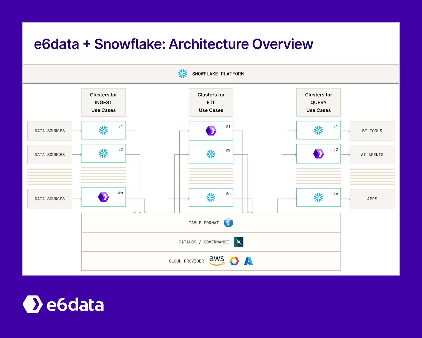
Alternatively, use e6data with Snowflake: 10x faster queries, 60% lower costs, no migration
If you’ve squeezed all the juice out of native Snowflake tuning and still need another step‑change, bolt e6data’s lakehouse query engine onto your Snowflake estate. You keep your data, your SQL, your governance model, and your BI tools- e6data simply takes over the heavy lifting on the toughest workloads.
e6data + Snowflake architecture overview diagram
Why teams add e6data on top of Snowflake
Why
How e6data delivers it
Business impact
10x faster SQL & AI workloads
Distributed, K8s‑native engine with atomic scheduling and advanced vectorized execution.
Sub‑second dashboards, even at 1000 QPS; interactive data exploration on TB‑scale sets.
Over 60% lower costs
Scales in single‑vCPU increments instead of leaping from M → L → XL. Pay only for cores you consume.
Free up $1.5‑10 M in annual Snowflake credits for the same workload.
Zero migration
Sits side‑by‑side with Snowflake; no data copy, no SQL rewrites, no catalog swap.
Add in days, not months—teams and dashboards stay online.
Iceberg & open‑format native
Reads Iceberg, Delta, Hudi straight from the lake; streams Kafka into Iceberg within 60s.
Unlock open‑table analytics without leaving Snowflake.
Multi‑region & hybrid ready
Affinity‑aware execution slashes cross‑cloud egress and latency.
One engine for on‑prem, AWS, Azure, GCP.
Getting started
Step
Action
Provision
Deploy e6data in your VPC or use its serverless option (marketplace images for AWS, Azure, GCP).
Connect catalogs
Point e6data at the same Hive/Glue/Unity catalog Snowflake sees; no duplicate schemas.
Redirect workload
In Snowflake, create an external function or use Snowflake Connector to send chosen queries to e6data; or route through BI tool DSNs.
Tune atomic scaling limits
Set min/max vCPUs per workload; e6data’s per‑CPU billing kicks in automatically.
Measure & iterate
Compare p95 latency and credit burn before/after—teams usually hit ROI in the first billing cycle.
When e6data makes the most sense
Massive spikes that push Snowflake warehouses to XXL for short windows.
High‑cardinality joins or large Iceberg tables where Snowflake pruning isn’t enough.
Multi‑cloud governance where data stays in multiple object stores, but users want a single SQL layer.
If those pain points sound familiar, pairing Snowflake with e6data can help a lot. For deeper architectural details and deployment guides, see e6data’s Snowflake‑compatibility overview.
.svg)


.svg)
.svg)
.svg)
.png)

.svg)
.svg)
.svg)
.svg)
.svg)