How to Optimize AWS Athena Costs? (2025 Edition)

‍

BI Dashboards

Dashboards often generate predictable, repetitive query patterns, and that makes them ripe for cost optimizations. 

‍

1. Cache duplicate dashboard queries with Result Reuse

Many BI tools use Athena with identical queries every few minutes, even if the underlying data hasn’t changed. All that redundant scanning piles up costs. 

For example, the Edge Delta team found that just 10 daily dashboard queries, each scanning ~0.55 TB, would rack up about $10K/year in Athena charges – and if those were hitting raw CSV data instead of optimized formats, it would have been over $30K/year. 

How to implement – 

• Athena’s Query Result Reuse feature will automatically cache query results and serve them on repeat executions of the exact same query (with the same input data). 
• In the Athena console, go to Workgroups → Settings → Result reuse, and set Result reuse to “Enforced = true” for your BI workgroup. You can also configure this via the API or CloudFormation. 

For example, using the AWS CLI to update a workgroup’s settings, you would include a JSON configuration like:

{
  "Enforced": true,
  "ResultReuseByAgeConfiguration": { "MaxAgeInMinutes": 60 }
}

‍

This ensures that if the same query text is executed again within 60 minutes (or whatever window you choose), Athena will skip the scan and return the cached results instantly (and for free).

Alternative – 

If your dashboards can’t use Athena’s built-in reuse (for instance, if queries aren’t exactly identical each time), consider using materialized views. Create a materialized view that pre-computes the expensive query, refresh it nightly or hourly, and point the dashboard to that view. The view acts as a cache of the latest results without repeatedly scanning the base table.

Takeaway – Cache first; pay to scan only when the data actually changes.

‍

2. Put a daily byte budget on your Athena workgroup

Every Athena query is billed for scanning at least 10 MB of data, even if it returns only a few rows, which can lead to high costs. For instance, an interactive dashboard widget might let users run 30 quick queries in a row, each scanning 50 GB – that’s 1.5 TB scanned in minutes, or about $7.50 in cost before you blink. 

Placing an upper limit on how much data a workgroup can scan per query (and per day) can safeguard your costs.

How to implement –

• In the Athena console, under your Workgroup Data usage control, set both “Bytes scanned per query” and “Bytes scanned per day” quotas. 
• These can also be set via Infrastructure as Code; in AWS CloudFormation, for instance, use the property BytesScannedCutoffPerQuery for the workgroup.

Alternative – 

For more flexible alerting, you can complement (or substitute) hard limits with CloudWatch Alarms. Monitor the AthenaDataScanned CloudWatch metric and set an alarm to trigger if daily scanned bytes approach your budget. 

Takeaway – Hard limits guardrails you against unnecessary large scan queries.

‍

3. Adopt Partition Projection instead of endless Hive folders

Traditional Hive-style partitioning (explicitly adding partitions to the Glue Catalog) can become a maintenance headache for large datasets, and if partitions are not added or updated in time, queries may end up scanning entire tables. 

Partition Projection lets Athena auto-discover partitions based on filename patterns, eliminating manual “MSCK REPAIR” runs and ensuring queries only read relevant slices of data. 

How to implement – 

• Partition projection is configured via table properties. You define the partition key patterns and value ranges up front, so Athena can infer partition locations on the fly. 
• For example, suppose you have an events table partitioned by date (year/month/day) in the S3 path. You can enable projection with an ALTER TABLE command:

‍

ALTER TABLE events
SET TBLPROPERTIES (
  'projection.enabled'='true',
  'projection.date.format'='yyyy/MM/dd',
  'projection.date.range'='2024/01/01,NOW',
  'projection.date.interval'='1',
  'projection.date.unit'='DAY',
  'storage.location.template'='s3://<your-bucket>/events/date=#{date}'
);

‍

• This tells Athena that events are partitioned by a date key following the format YYYY/MM/dd, ranging from Jan 1, 2024, through the current day. It also provides a template for the S3 path. 
• With this config, you no longer need to run MSCK REPAIR TABLE or add partitions manually – Athena will assume partitions exist for each date in range and only read the ones relevant to your query’s WHERE date = '2024-12-01' clause, for example.

Alternative – 

• For legacy datasets where re-partitioning or projection is hard to implement, look into Glue Partition Indexes. A partition index in Glue can speed up queries on heavily partitioned tables by indexing the partitions, reducing the overhead of discovering them. This still requires keeping partitions up to date, but can mitigate some performance cost of large partition sets when you cannot use projection.
• Consider migrating to an alternative engine for the select workload that demands high performance at manageable costs. e6data’s compute engine, for instance, implements partitioning logics automatically due to its architecture (amongst other things) and therefore, can be up to 70-90% faster than Athena for high-performance workloads at lower costs.

Takeaway – Partition Projection delivers the benefits of partition pruning with zero metastore upkeep, no more forgotten partitions or full-table scans by accident.

‍

4. Compress and auto-purge query result files

Athena’s query results are written to S3, and they can incur sneaky hidden costs if unmanaged. 

• First, if you leave the default CSV/JSON result format, those files are larger than necessary (uncompressed), meaning more storage cost and higher GET request latency. 
• Second, the accumulation of result files over months or years can silently cost you in S3 storage and retrieval fees. 

How to implement – 

• Use compressed, columnar formats for query results: In the Athena web console, when you run a query, you can choose the result format. Switch from the default CSV to a compressed format like Apache Parquet or ORC, or at least GZIP-compressed CSV. If using the API or JDBC, set the ResultConfiguration to specify Parquet or GZIP for compressionType. This can shrink each result file dramatically, especially if your results have repetitive text.
  
  
• Apply an S3 Lifecycle policy to Athena results: Set your AthenaQueryResults/ S3 prefix to auto-delete or auto-archive files after a short period (e.g., 3 days or 1 week). Most Athena query results are only needed immediately by the application or user; after a few days, they’re rarely accessed again. For example, you can attach a lifecycle rule like:

‍

<Rule>
    <Prefix>AthenaQueryResults/</Prefix>
    <Status>Enabled</Status>
    <Expiration>
        <Days>3</Days>
    </Expiration>
</Rule>

‍

Alternative – 

• If certain teams require longer retention of query outputs (e.g., for compliance or re-use), consider using S3 Intelligent-Tiering storage class for the results bucket or prefix. Intelligent-Tiering will automatically move objects to cheaper storage tiers as they age, reducing cost without fully deleting the data. 
• Another approach is to periodically archive old results to Glacier Instant Retrieval (which we discuss later for cold data storage).

Takeaway – Smaller, short-lived result files ensure S3 costs don’t end up out-billing your Athena queries.

‍

5. “Burst” with Provisioned Capacity only for peak hours

Athena offers Provisioned Capacity dedicated DPUs) to handle high query volumes or concurrency beyond the on-demand limits. It costs $0.30 per DPU-hour (billed per minute), which can be cost-effective for heavy, constant workloads.

However, it’s easy to leave provisioned capacity running 24/7 even if only truly needed for a morning rush. For example, imagine you allocate 20 DPUs for your BI dashboards. That’s $6/hour, or ~$144/day. If those dashboards really hammer Athena only from 9 a.m. to 11 a.m. each day, the other 22 hours are mostly idle, potentially wasting over $100/day. 

How to implement – 

Allocate provisional capacity during known busy times and deallocate (scale to zero) when not needed. In the Athena console, you can pre-create a Capacity Reservation (e.g., 20 DPUs named “bi_capacity”). Then use a script or AWS SDK (boto3, etc.) to scale the allocated DPUs up or down. 

Alternative – 

• If you prefer not to manage schedules, another approach is to stagger your dashboard refresh times so that the default on-demand Athena can handle them within the concurrency limit.
• You can also use an alternative engine for high-concurrency workloads alone. e6data’s compute engine can fit right on top of S3 and handle concurrency up to 1000 QPS at up to 60% lower costs. As the engine is disaggregated and distributed, the services are run at once (instead of queuing) and the billing is per CPU (i.e. cores consumed) instead of uptime. 

Takeaway – Provision capacity when you need a feast of queries, but don’t pay for it 24/7.

‍

6. Pre-aggregate “hot” metrics overnight

Dashboard queries that have to sum or process millions of raw rows for each load are inherently expensive. If your dashboards frequently query very granular data (e.g., raw event logs) to compute higher-level metrics, you’re essentially redoing heavy computations and scans on each refresh. 

How to implement – 

Identify the “hot metrics” or common groupings your dashboards use (e.g., total sales by day). Create a scheduled job to run a CTAS (Create Table As Select) query that aggregates your raw data into a new table. 

For instance:

-- Nightly batch job to aggregate yesterday’s events into summary table
CREATE TABLE bi_rollups
WITH (format = 'PARQUET', compression = 'SNAPPY') AS
SELECT date, country, SUM(sales) AS total_sales, COUNT(*) AS order_count
FROM raw_events
WHERE date = date '2025-01-15'  -- or whatever date partition or range
GROUP BY date, country;

‍

• This creates a bi_rollups Parquet table partitioned by date, with one row per country per day, instead of potentially millions of rows of raw events. 
• Adjust the grouping keys and timeframe as needed for your use case (you might roll up by day, by week, etc.). Each morning, your dashboards can query bi_rollups for yesterday’s metrics with negligible cost.

‍

Alternative – 

Athena now supports Materialized Views, which can achieve a similar result with potentially less manual orchestration. 

You could create a materialized view like CREATE MATERIALIZED VIEW daily_sales AS SELECT date, country, SUM(sales) ... and have it refresh automatically or on a schedule. The view will maintain the pre-aggregated data for you. 

Takeaway – Scan MBs, not TBs, on every dashboard render. By pre-computing common metrics, your dashboards read tiny summary files instead of entire raw datasets each time.

‍

Ad-hoc Querying

These one-off or iterative queries can be Athena’s greatest strength, but they also open the door to inadvertent inefficiencies – e.g., scanning a multi-terabyte table just to test a hypothesis, or running the same expensive join repeatedly during development.

1. Flip on the Cost-Based Optimizer (CBO)

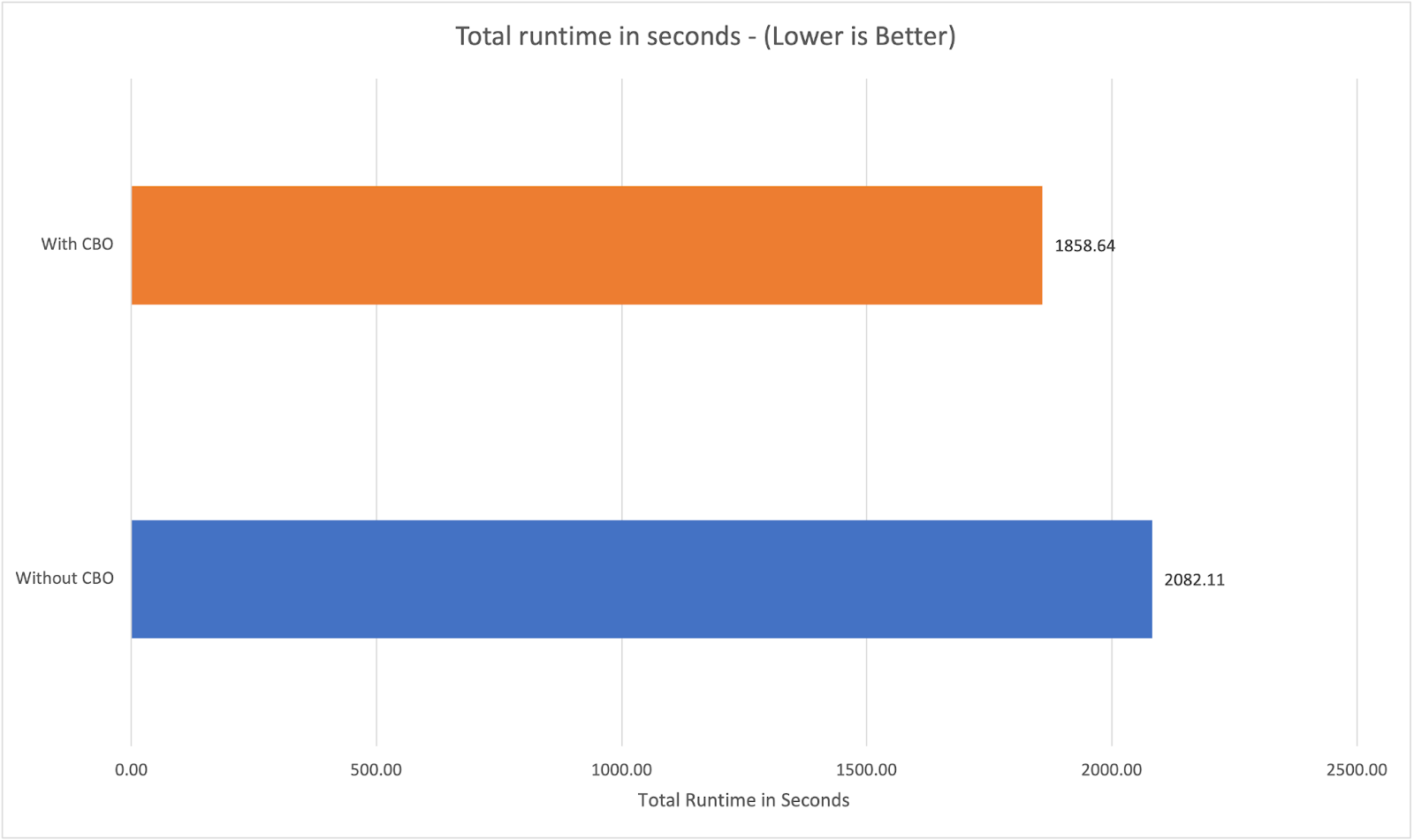
Athena’s newer engine versions include a Cost-Based Optimizer that can dramatically improve query efficiency by making smarter decisions on join order, data scanning, and aggregation pushdown – if it has table statistics available. 

AWS’s own benchmarks showed that enabling the CBO made some complex queries up to 2x faster, and overall query runtime dropped by ~11% on a standard TPC-DS workload. 

How to implement – 

First, ensure you’re using Athena engine version 3 (which has CBO capabilities). Next, generate statistics for your frequently queried tables: in Athena, you do this by running the ANALYZE command. For example:

‍

ANALYZE TABLE sales COMPUTE STATISTICS;

‍

This tells Glue to compute column statistics (like min, max, NDV, etc.) for the sales table, which Athena’s optimizer will use for planning. Do this for your large or important tables (you can target specific columns or the whole table).

Athena’s CBO is automatically used when stats exist, but you can double-check or force it by setting a session property:

SET SESSION join_reordering_strategy = 'AUTOMATIC';

‍

If you’re using JDBC/ODBC or notebooks, ensure this session property is on or use the equivalent toggle.

Alternative – 

• In cases where you cannot easily gather stats (maybe the data is too volatile or you’re on an older engine version), you’ll have to rely on manual query tuning. Use EXPLAIN on your queries to see the plan and identify if a large table is being joined or scanned earlier than it should. You might rewrite the SQL to join or filter in a better order yourself. This is essentially doing the optimizer’s job by hand – tedious, but can be worthwhile for extremely large queries if CBO isn’t an option.
• You can also offload these select workloads to an alternative engine like e6data, which is specifically highly performant on complex SQL queries (like with large table scan volume, high-cardinality joins, etc.) at lower costs.

Takeaway – One ANALYZE today can mean perpetual savings thereafter. Investing in table stats and the CBO makes Athena automatically do less work for the same answers.

2. Surface the data scanned for every query (to the user)

When analysts run queries interactively, they often focus only on the result, not realizing how much data was scanned. By making query cost visible for each query, you nudge users to be mindful. 

How to implement – 

• In notebooks or custom applications: If users query Athena via a Jupyter notebook (Python) or custom script, you can use the AWS SDK to retrieve scanned bytes after each query and display them.
  
  
• In the Athena console, the Athena web console now has an option to “Display query metrics,” which includes data scanned. Encourage your team to toggle this on, or use Athena Workgroups with metrics and have users check the History pane for scanned data after running a query.

Alternative – 

For a quick solution, you can also leverage CloudWatch Logs Insights if you have Athena’s execution logs enabled. You could query Athena’s own logs to find queries and their scanned bytes, and then share a dashboard of that. It’s not real-time per query, but it can reveal trends.

Takeaway – Visible cost = mindful analysts. When users see the “price” of each query, they naturally learn to be more efficient.

‍

3. Stage heavy joins with CTAS + Parquet

When working on analyses, users often join the same large tables multiple times as they iterate. Each time, Athena scans those tables in full. A smarter approach for repetitive joins or complex subqueries is to do it once, store the result, and then query that instead.

How to implement – 

Let’s say you’re repeatedly querying a combination of tables or applying the same complex filter criteria. Do it once and materialize the results. You can use a CTAS query in Athena to create a temporary table. For example:

‍

CREATE TABLE scratch.joined_data
WITH (format = 'PARQUET', compression = 'SNAPPY') AS
SELECT a.user_id, a.event_time, b.purchase_amount, c.country
FROM raw_events a
JOIN purchases b ON a.event_id = b.event_id
JOIN users c ON a.user_id = c.user_id
WHERE a.event_time >= '2025-01-01' 
  AND b.purchase_amount > 0;

‍

Alternative – 

For quick one-off filtering of a single large file, consider Amazon S3 Select. If your data is in CSV/JSON and you want to retrieve a subset of columns or rows from one object, S3 Select can pull just that subset (reducing data transfer) without Athena overhead. It’s not suitable for joins or large multi-file operations, but for simple “select a few columns from this giant file” tasks, it can be cheaper and faster.

Takeaway – Pay once; read fast forever. Doing a heavy join or filter once and reusing the results means you pay the scan cost one time and then enjoy quick, cheap queries thereafter.

‍

4. Separate “read” and “write” workgroups

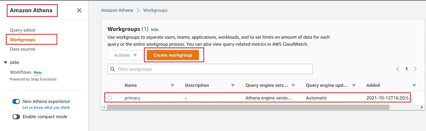
Athena’s performance (and cost) can degrade if too many queries contend for resources in one workgroup. Notably, long-running ETL or insert jobs can clog up the queue and slow down interactive queries. This way, an analyst isn’t waiting behind a huge batch job, and if needed, you can allocate separate capacity policies to each.

How to implement – 

Athena Workgroups are your friend here:

• Create two workgroups, for example analytics_ro (read-only / BI / analyst usage) and data_pipeline_rw (for ETL, writes, CTAS, etc.). 
• Assign users or applications to use the appropriate workgroup – for instance, when using the JDBC/ODBC driver or the AWS SDK, there’s a parameter to specify the workgroup. 
• In AWS SDK or CLI, it might look like --work-group data_pipeline_rw for your pipeline scripts. In BI tools like Quicksight or others, configure one data source to use the read-only workgroup for queries.
• Within Athena, you can also set different settings per workgroup: e.g., the ETL workgroup might have no query caching, whereas the analytics one has result reuse on. 

‍

‍

Alternative – 

For an even stronger isolation, some organizations create a dedicated AWS account for analysts and a different account for data engineering jobs. Athena’s cost is then isolated by account. Cross-account S3 access can let the analysts query the data without being impacted by the ETL account’s Athena usage at all. This is a heavier setup (requires managing two accounts and permissions), so using two workgroups is the simpler first step.

Takeaway – No more BI users queued behind nightly batch loads. Isolating workloads ensures a rogue ETL job can’t throttle your interactive queries (and vice-versa).

‍

5. Auto-delete (or archive) old result sets

This might sound familiar from the BI section: ad-hoc queries also produce result files, and often even more chaotically. An analyst might run hundreds of throwaway queries in a day, generating hundreds of small S3 files. Over time, without cleanup, you accumulate potentially millions of objects consuming space and incurring request costs. 

How to implement – 

• The solution is the same S3 lifecycle approach: apply a rule on the bucket/prefix used for Athena results to delete objects after, say, 3 days. If you have a dedicated results bucket, you can apply a bucket-wide rule. If not, you can target the specific prefix (e.g., athena-results/analysts/).
• If outright deletion is too aggressive for your needs, you could instead transition older results to a cheaper storage class like Glacier Instant Retrieval after 30 days, so they cost almost nothing unless retrieved (and if you do need an old result, Athena can still query Glacier IR objects directly with a slightly higher cost).

Alternative – 

Instead of relying on S3 lifecycle alone, you could incorporate a cleanup step in your workflow. For instance, run a daily AWS Lambda that finds and deletes Athena result objects older than X days, or have users run queries in a scratch workgroup whose results bucket is periodically purged. This offers more control (you might skip deleting certain important query outputs), but it’s more work to maintain. 

Takeaway – Treat Athena result sets as temporary scratch data – they shouldn’t outlive their usefulness. 

‍

6. Replace SELECT * with pruned, safe views

SELECT * in Athena means scan every column of every row – you’ll pay to read all the data, even the columns you don’t actually use. An analyst might do SELECT * FROM large_table LIMIT 100 just to see the schema or a sample, but Athena will still scan potentially gigabytes or more, only to return 100 rows. 

How to implement – 

Encourage a culture (and provide tools) to select only needed columns. A practical way is to create safe, column-pruned views for commonly accessed tables. For example, if analysts only need a subset of columns from a raw events table, create a view that exposes just those:

‍

CREATE VIEW safe_events AS
SELECT id, event_ts, country, device, ...  -- (list only useful columns)
FROM raw_events;

‍

Alternative – 

Some teams leverage third-party tools or even custom Athena UDFs as a linter. Another approach is using Athena query federation to a proxy that can block certain patterns. These are complex solutions; a well-placed convention and view are usually sufficient.

Takeaway – By providing pre-defined, narrower views or simply instilling the habit of specifying columns, you can dramatically cut down scanned data (and costs).

‍

ETL / Data Pipelines

Pipeline workloads can become one of the biggest cost drivers if not optimized: they might run on large raw datasets, produce multiple outputs, or use provisioned capacity for throughput. 

‍

1. Write Snappy-compressed Parquet, not raw CSV

The format you store your data in has an enormous impact on Athena costs. Text formats like CSV or JSON are bulky; Athena has to scan every byte of them. Columnar formats like Parquet or ORC, especially with compression, shrink the data to be scanned and allow Athena to skip irrelevant columns.

For ETL jobs that produce new tables, choosing Parquet+compression will make all downstream queries dramatically cheaper (and faster).

How to implement – 

Whenever you have an Athena CTAS (Create Table As) or INSERT INTO that materializes data, specify a columnar format and compression. For example, in Athena SQL:

‍

CREATE TABLE cleaned_data
WITH (format='PARQUET', compression='SNAPPY') AS
SELECT *
FROM staging_raw_data;

This reads staging_raw_data (perhaps in CSV or raw form) and writes it out as a new table cleaned_data, in Parquet format compressed with Snappy. Snappy is a good default compression for Parquet in Athena – it’s fast and gives decent compression. You could also use GZIP for higher compression at the cost of slower performance. 

The key is not leaving data in plain text once it’s been processed. If you have existing pipelines writing to S3 via Glue jobs or Spark, configure those sinks to use Parquet or ORC. The one-time conversion cost pays for itself quickly in query savings.

Alternative – 

• If your workload is append-only and query latency isn’t super sensitive, ORC with ZSTD compression can sometimes yield even smaller file sizes than Parquet/Snappy (meaning even lower scan costs). 
• ORC is another columnar format that Athena supports well. ZSTD is a compression algorithm offering high ratios. The trade-off is that reading ZSTD-compressed ORC can be a bit slower CPU-wise, but if your priority is minimizing bytes scanned (e.g., in a very large archive dataset), it’s worth considering.

Takeaway – Smaller files = faster scans = tinier bills. Use columnar formats and compression so Athena reads gigabytes instead of terabytes for the same data.

‍

2. Balance partitions with buckets for high-cardinality keys

Partitioning is great for pruning large swaths of data, but if you partition on a very high-cardinality column (like user_id), you can end up with millions of tiny partitions, which hurts performance and incurs overhead. On the flip side, not partitioning that data means each query has to scan all the data for a given user. 

The solution is bucketing: it groups data by a key into a fixed number of buckets (files) such that queries filtering on that key only scan a subset of buckets, not every file.

How to implement – 

When creating tables in Athena, you can specify bucketing (also known as clustering in the CREATE TABLE syntax). Suppose we have a large transactions table of user events. We might partition it by date (daily partitions), but also bucket by user_id to distribute each day’s data into, say, 32 buckets by user. For example:

‍

CREATE TABLE transactions_bucketed
PARTITIONED BY (dt string)
CLUSTERED BY (user_id) INTO 32 BUCKETS
AS
SELECT * 
FROM transactions_raw;

‍

This CTAS will reorganize the data such that for each dt partition, there are 32 files, each containing a range of user_id hash values. When Athena later queries transactions_bucketed for a specific user_id (or a small set of users), it can skip most of those buckets, scanning only 1/32 of the data (in this example). 

Bucketing in Athena requires using the same number of buckets consistently, and queries use equality filtering on the bucket column to benefit. But when they do, it’s a big win.

Alternative – 

• Athena engine version 3 supports Iceberg tables with hidden partitioning. Iceberg can automatically organize data by partition keys and even do something akin to bucketing under the hood (it can cluster data by partition spec). If you use Iceberg (discussed next), some of these concerns can be handled by Iceberg’s metadata instead of manual bucketing. Still, plain bucketing is available on non-Iceberg tables and works well if you plan it upfront.
• If your Athena version doesn’t support Iceberg, consider offloading these select workloads to one that does. e6data’s compute engine is built with native and advanced Iceberg support and can get you started instantly without migration overhead. 

Takeaway – Evenly sized files and buckets lead to consistent, efficient scans. Bucketing prevents the “too many tiny partitions” problem while still limiting scan scope for high-cardinality filters.

‍

3. Use Apache Iceberg for mutable or rapidly evolving datasets

Athena traditionally works best with append-only, static datasets. If you have datasets that require updates, deletes, or frequent schema changes, using normal Glue tables means you often have to rewrite entire partitions or maintain complicated pipelines. 

This can be costly – rewriting a whole partition just to change a few records means rescanning and rewriting a lot of data. Iceberg enables merge-on-read and hidden partitioning, meaning you can upsert or delete data in place without horrific reprocessing costs. With Iceberg, small incremental changes don’t require full table scans to be queryable.

How to implement – 

Athena can create and query Iceberg tables natively (engine version 3). To convert or create a dataset as Iceberg, you use a CREATE TABLE statement with table_type='ICEBERG'. For example, say you have daily updates coming in for a sales table – rather than maintain a separate “delta” table and then merge it, you can do:

‍

CREATE TABLE sales_iceberg
WITH (table_type='ICEBERG', format='PARQUET')
AS 
SELECT * 
FROM sales_updates;

‍

This will create sales_iceberg as an Iceberg table (stored in Parquet under the hood) and import the data from sales_updates. 

Going forward, you could use MERGE INTO or DELETE statements on sales_iceberg to apply changes. Iceberg handles versioning and only reads the portions of data necessary for queries via metadata. It also automatically tracks partitions (you can even partition by transformed keys, like year/month or truncate timestamps, without predefining folder paths). 

Alternative – 

• If your priority is query speed on updated data, Hudi copy-on-write might be a fit (at the cost of more write-time overhead). If you need faster writes, Hudi’s merge-on-read is akin to Iceberg’s approach. 
• Generally, Iceberg has become quite popular for Athena due to its strong compatibility and feature set, but Hudi is an option, especially if you’re already using it in Spark or other tools.

Takeaway – By using modern table formats designed for mutability (like Iceberg), you avoid re-scanning or rewriting huge datasets for small changes, thereby saving tons of compute (and money).

‍

4. Tier cold data to cheaper storage (Glacier) for long-term retention

Athena charges you for every byte scanned, regardless of S3 storage class. However, your S3 storage costs themselves can be optimized. 

Many ETL pipelines produce data that is very hot when first created (queried often for recent reports), but then goes cold. Months or years of historical data might rarely be queried, yet you pay full price to store it in S3 Standard. 

By tiering older data to Glacier Instant Retrieval (Glacier IR) or other archival storage, you cut storage costs by up to 90% – Glacier IR costs around $0.004 per GB-month (one-tenth of S3 Standard) and still allows direct Athena queries on the data when needed, with just a small per-query retrieval fee. 

How to implement – 

• Use S3 Lifecycle rules on your data lake buckets to transition objects to cheaper tiers as they age. 
• Glacier IR objects can be read by Athena without a restore step (they incur a ~$0.003 per 1000 requests and $0.12/GB retrieval fee, which will slightly increase the per-query cost when querying archived data – but if it’s infrequent, it’s negligible compared to always keeping in Standard). 
• If you have a disaster recovery requirement, another angle is to replicate data to a cheaper region and archive it there. For instance, if you must keep 7 years of data, keep the latest year in primary region S3 Standard, move older years to S3 Glacier in a less expensive region (us-west-2 vs us-east-1, etc. – pricing can differ). Athena can query across regions if needed (with some data transfer costs), or you can temporarily restore data for analysis.
• You can also consider using a hybrid, locality-aware compute engine like e6data, which can separate compute from compute owing to its kubernetes-based architecture and therefore offer egress fee as low as zero.

Alternative – 

• If Glacier IR’s retrieval fee is a concern, you could consider S3 Intelligent-Tiering, which will auto-tier objects to Archive tiers but bring them back if accessed (though with fees). It’s hands-off but slightly more costly than a well-planned lifecycle for Glacier classes. 
• Another alternative is compressing old data more aggressively (e.g., ZSTD) to at least reduce storage size if you prefer to keep it in S3 Standard for faster access.

Takeaway – Storage tiers are the stealth lever in long-term TCO. By sliding your cold data into cheaper storage, you cut costs without affecting Athena’s ability to query the data when needed.

‍

Explore e6data for Faster Queries & Lower Bills

Athena is terrific for ad-hoc discovery, but some workloads simply need more horsepower or finer-grained cost control than $5 / TB scans can deliver. That’s where e6data’s compute engine can complement (or even replace) parts of your Athena stack:

# 1️⃣ Launch an e6data workspace (web console or Terraform)
# 2️⃣ Attach your existing Glue Catalog and S3 buckets
# 3️⃣ Point your BI tool or JDBC string to jdbc:e6://<endpoint>
# 4️⃣ Run the same SQL—see results (and cost) side-by-side